Image super-resolution (SR) is a technique aiming at the estimation of a high-resolution (HR) image from one or several low-resolution (LR) observation images, which is widely used in remote sensing, biometrics identification, medical imaging, video surveillance, etc. There are three categories of super resolution methods. Interpolation methods are simple but short of high-frequency component, while reconstructed methods degrade rapidly when the desired magnification factor is large.

Recently, the third category called learning based methods are developed, which become the most active research area. In this method, a HR image can be predicted by learning the co-occurrence relationship between a set of LR example patches and corresponding HR patches. Standard methods are example based method^[1], neighbor embedding^[2], etc. Motivated by compressive sensing theories^[3], Ref.[4] proposed an algorithm which used sparse representation of the input LR image to reconstruct the corresponding HR image with two jointly trained dictionaries. The method used the inherent data message, mapped the data in some dictionaries, and reflected the data information by some sparse coefficients, which turned out to reconstruct the HR image greatly.

There are many classic sparse representation methods. Greedy methods, like orthogonal matching pursuit (OMP^[5]), attack the problem heuristically by fitting the sparse models using greedy stepwise least squares. But they are often computationally slow. The least angel regression (LARS^[6]) algorithm adds a new element to the active set of nonzero coefficients by taking a step along a direction having equal angles with the vectors in the active set at each iteration. But when the iteration number is large, the method is not efficient. Preconditioned conjugate gradients (PCG^[7]) uses the internal Newton's method to minimize the logarithmic barrier function and receives good results. But it is time-consuming.

In this paper, the feature sign method for single image SR via sparse representation is proposed which can overcome above drawbacks. By determining the sign of the sparse coefficients, the non-differentiable problem is changed to an unconstrained quadratic optimization problem (QP) which can be solved easily. It is competent to capture the sparse coefficient of data in an over-completed dictionary efficiently and rapidly. Simulation results demonstrate that it obtains better reconstruction performance qualitatively and quantitatively over other classic SR methods.

1 Single Image SR Using Sparse Representation

The super-resolution image reconstruction problem is known to be an ill-posed inverse problem. Various approaches have been proposed to regularize it, while they all share two parts of constraints priors:

$\mathit{\boldsymbol{U}}(x) = \left\| {y - \mathit{\boldsymbol{H}}x} \right\|_2^2 + \lambda \mathit{\boldsymbol{E}}(x)$

(1)

where $\mathit{\boldsymbol{H}}$ is reconstruction error constraint which represents data-fidelity, and $\lambda $ is sparsity prior constraint which represents the desired sparse properties of the HR images. For the latter one, most explicit regularization techniques enforce ${\ell _0}$ -, ${\ell _1}$ - or ${\ell _2}$ -minimization properties of the HR image $\mathit{\boldsymbol{X}}$, thus resulting in many different sparse algorithms.

In this paper, the ${\ell _1}$ -minimization is taken to calculate the sparse coefficient, which has been proved by Ref.[8] as long as the sparse representation coefficients of the ${i^{{\rm{th}}}}$ patch ${\alpha _i}$ are sufficiently sparse, and the NP-hard problem can be efficiently solved by minimizing the ${\ell _1}$ -norm:

$\min {\left\| {{\alpha _i}} \right\|_1}{\rm{s}}{\rm{.t}}{\rm{.}}\left\{ \begin{array}{l} \mathit{\boldsymbol{F}}\left\| {{\mathit{\boldsymbol{Z}}_l}{\alpha _i} - {y_i}} \right\|_2^2 \le {\varepsilon _1}\\ \mathit{\boldsymbol{F}}\left\| {{x_i} - {\mathit{\boldsymbol{Z}}_h}{\alpha _i}} \right\|_2^2 \le {\varepsilon _2}\\ \left\| {\mathit{\boldsymbol{R}}{\mathit{\boldsymbol{Z}}_h}{\alpha _i} - \mathit{\boldsymbol{v}}} \right\| \le {\varepsilon _3} \end{array} \right.$

(2)

where $\mathit{\boldsymbol{F}}$ is an identity matrix or a linear feature extraction operator. It can be some kind of high-pass filter, for example, the first-order and second-order derivatives. Matrix $\mathit{\boldsymbol{R}}$ extracts the region of overlap between current target patch and previous reconstructed HR image, and $v$ contains the values of the previous reconstructed HR image on the overlap. Formula (2) ensures that the obtained coefficient ${\alpha _i}$ can best extract sparse information of $\mathit{\boldsymbol{Y}}$ in ${\mathit{\boldsymbol{ Z}}_l}$, and so can be used to reconstruct $\mathit{\boldsymbol{ X}}$ with ${\mathit{\boldsymbol{ Z}}_h}$.

The SR algorithm is a patch-wise based sparse recovery with the joint learning dictionaries. The input LR image $\mathit{\boldsymbol{ Y}}$ is interpolated to the size of desired HR image at first, and then divided into a set of overlapping patches of size $p \times p$. For each LR image patch ${y_i}$, the feature $y$ is extracted in the training phase, and sparse representation ${\alpha _i}$ is computed with respect to low-resolution dictionary ${\mathit{\boldsymbol{ Z}}_l}$. ${\alpha _i}$ is then used to predict the underlying HR image patch ${x_i}$ (feature $x$) with respect to high-resolution ${\mathit{\boldsymbol{ Z}}_h}$. The predicted HR patches are tiled together to reconstruct the HR image $\mathit{\boldsymbol{ X}}$.

In this work, the pair of over-complete dictionary $\{ {\mathit{\boldsymbol{ Z}}_h},{\mathit{\boldsymbol{ Z}}_l}\} $ are jointly trained^[9] by using the K-SVD^[10] method:

$\begin{array}{l} \mathop {\min }\limits_{{\mathit{\boldsymbol{Z}}_h},{\mathit{\boldsymbol{Z}}_l},\{ {\alpha _i}\} _{i = 1}^N} \sum\limits_{i = 1}^N {(\left\| {{x_i} - {\mathit{\boldsymbol{Z}}_h}{\alpha _i}} \right\|_2^2} + \left\| {{y_i} - {\mathit{\boldsymbol{Z}}_l}{\alpha _i}} \right\|_2^2) + \lambda {\left\| {{\alpha _i}} \right\|_1}\\ \;\;\;\;\;\;\;\;\;\;{\rm{s}}{\rm{.t}}{\rm{.}}\;\;\;\;{\left\| {{\mathit{\boldsymbol{Z}}_x}(:,k)} \right\|_2} \le 1,{\left\| {{\mathit{\boldsymbol{Z}}_y}(:,k)} \right\|_2} \le 1 \end{array}$

(3)

2 Feature Sign Method

How to solve formula (2) fast and efficiently is the fundamental of sparse representation and quality determination of reconstructed HR image. It is a typical ${\ell _1}$ -regularized least squares problem which can be solved by many sparse algorithms.

To keep it simple, it can be rewritten in a vector form as:

${\min _\alpha }\sum\limits_{i = 1}^m {\left\| {{y_i} - \mathit{\boldsymbol{Z}}{\alpha _i}} \right\|_2^2} + \lambda \sum\limits_{i = 1}^m {{{\left\| {{\alpha _i}} \right\|}_1}} $

(4)

Let ${\alpha _i}^{(j)}$ be the ${j^{{\rm{th}}}}$ coefficient of ${\alpha _i}$, then the optimization problem is equal to:

${\min _{{\alpha _i}}}p({\alpha _i}) = \left\| {{y_i} - \mathit{\boldsymbol{Z}}{\alpha _i}} \right\|_2^2 + \lambda \sum\limits_{j = 1}^k {\left| {{\alpha _i}^{(j)}} \right|} $

(5)

If the sign of ${\alpha _i}^{(j)}$ at each iteration is known, then the non-differentiable problem can be changed to an unconstrained quadratic optimization problem (QP) which can be solved easily.

The sign can be settled by 4 steps:

1) Define $p({\alpha _i}) = \left\| {{y_i} - \mathit{\boldsymbol{Z}}{\alpha _i}} \right\|_2^2 + \lambda |{\alpha _i}^{(j)}|$ and set $f({\alpha _i}) = \left\| {{y_i} - \mathit{\boldsymbol{Z}}{\alpha _i}} \right\|_2^2$, $g({\alpha _i}) = \lambda |{\alpha _i}^{(j)}|$. Define ${\nabla _i}^{(j)}|{\alpha _i}|$ as the sub-differentiable value of the ${j^{{\rm{th}}}}$ coefficient of ${\alpha _i}$.

2) If $|{\alpha _i}^{(j)}| > 0$, ${\nabla _i}^{(j)}|{\alpha _i}|$ is given by the sign of ${\alpha _i}^{(j)}$. If ${\alpha _i}^{(j)} = 0$, then the sub-differentiable value ${\nabla _i}^{(j)}|{\alpha _i}|$ is given from the set of $[ - 1,1]$.

3) So the optimality conditions for achieving the optimal value of $p({\alpha _i})$ are translated to

$\left\{ \begin{array}{l} {\nabla _i}^{(j)}f({\alpha _i}) + \lambda {\rm{sign}}({\alpha _i}^{(j)}) = 0\;\;\;\;{\rm{if}}\;\left| {{\alpha _i}^{(j)}} \right| > 0\\ \left| {{\nabla _i}^{(j)}f({\alpha _i})} \right| \le \lambda \;\;\;\;\;\;\;\;\;\;\;\;\;\;\;\;\;\;\;\;\;{\rm{if}}\;{\alpha _i}^{(j)} = 0 \end{array} \right.$

(6)

4) Consider how to select the optimal sub-gradient ${\nabla _i}^{(j)}g({\alpha _i})$ when the optimality conditions are violated. Consider the case where $|{\nabla _i}^{(j)}f({\alpha _i})| > \lambda {\kern 1pt} {\kern 1pt} {\kern 1pt} $ and ${\kern 1pt} {\kern 1pt} {\alpha _i}^{(j)} = 0$. Suppose ${\nabla _i}^{(j)}f({\alpha _i}) > \lambda $, which means ${\nabla _i}^{(j)}p({\alpha _i}) > 0$. In order to decrease $p({\alpha _i})$, ${\alpha _i}^{(j)}$ must be decreased. Since ${\alpha _i}^{(j)}$ is now at the null point, the very first decrease to ${\alpha _i}^{(j)}$ is changing it to a negative number. So set ${\rm{sign}}({\alpha _i}^{(j)}) = - 1$. Similarly, if $|{\nabla _i}^{(j)}f({\alpha _i})| < - \lambda $, then set ${\rm{sign}}({\alpha _i}^{(j)}) = 1$.

3 Compute Sparse Coefficients

The algorithmic procedure of learning coefficients using feature sign is described in the following 5 steps.

An active set $\mathit{\boldsymbol{H}} \triangleq \{ j|\alpha _i^{(j)} = 0,|\nabla _i^{(j)}f({\alpha _i})| > \lambda \} $ is maintained for potentially nonzero coefficients and their corresponding signs $\mathit{\boldsymbol{\beta}} = [{\beta} _1,{\beta _2}, \cdots ,{\beta _k}]$, the image point $y = [{y_1},{y_2}, \cdots ,{y_n}]$, the dictionary is $Z$, and sparse parameter is $\lambda $.

1) Initialize: ${\alpha _i} = \mathit{\boldsymbol{0}},\mathit{\boldsymbol{\beta}} = \mathit{\boldsymbol{0}},\mathit{\boldsymbol{H}} = \phi $, ${\mathit{\boldsymbol{\beta}} _j} \in \{ - 1,0,1\} $ denotes sign(${\alpha _i}^{(j)}$);

2) Activate: From zero coefficient of ${\alpha _i}$, select $j = \arg {\max _j}|{\nabla _i}^{(j)}f({\alpha _i})|$. Activate ${\alpha _i}^{(j)}$ (add $j$ to the active set H) only if it locally improves the objective (6);

3) Feature sign: Let $\hat{ \mathit{\boldsymbol{Z}}}$ be a sub-matrix of Z that contains only the columns corresponding to the active set of ${\alpha _i}$ and ${f_i}$, and $\hat{ \mathit{\boldsymbol{\beta}}} $ be $\mathit{\boldsymbol{\beta}} $ corresponding to the active set. Compute the solution to the resulting unconstrained QP problem:

$\min p({\hat \alpha _i}) = ||{y_i} - \mathit{\boldsymbol{\hat Z}}{\hat \alpha _i}||_2^2 + \lambda {\mathit{\boldsymbol{\hat \beta }}^{\rm{T}}}{\hat \alpha _i}$

(7)

Let $(\partial p({\hat \alpha _i})/\partial {\hat \alpha _i}) = 0$, the optimal value of ${\alpha _i}$ under the current active set is:

${\hat \alpha _i}^{{\rm{new}}} = {({\mathit{\boldsymbol{\hat Z}}^{\rm{T}}}\mathit{\boldsymbol{\hat Z}})^{ - 1}}({\mathit{\boldsymbol{\hat Z}}^{\rm{T}}}{y_i} - \lambda \mathit{\boldsymbol{\hat \beta }})$

(8)

Perform a discrete line search on the closed line segment from ${\hat \alpha _i}$ to ${\hat \alpha _i}^{{\rm new}}$ : Check the objective value at ${\hat \alpha _i}^{{\rm new}}$ and all points where any coefficient changes sign, and update ${\hat \alpha _i}$ (and the entries in ${\alpha _i}$) to the point with the lowest objective value. Remove zero coefficients of ${\hat \alpha _i}$ from the active set and update $\mathit{\boldsymbol{\beta}} $ = sign(${\alpha _i}$);

4) Check the optimality conditions: Check the optimality conditions based on formula (6);

5) Output: The optimal coefficient matrix is ${\mathit{\boldsymbol{\alpha}} ^ * } = [{\alpha _1}^ * ,{\alpha _2}^ * , \cdots ,{\alpha _m}^ * ]$.

4 Experiment Results

In the following section, simulation results are given to illustrate the performance of our scheme. The simulation and comparison are carried out by Matlab implementations. All experiments are executed on a 2.33 GHz Intel Core 2 Quad CPU Q8200 processor with 2 GB memory in Windows XP OS.

This paper samples 20 000 HR and LR patch pairs from the training images to learn the over-complete dictionary randomly. $\lambda $ is 0.15 and the dictionary size is 1 024 in all experiments, which is proved to the best suitable number to balance between computation complexity and image quality. The input LR images are magnified by a factor of 3. The input patches are 5×5 pixels with an overlap of 3 pixels. For color images, the SR algorithm is only applied on the Y (intensity) channel, and the Cb and Cr chromatic channels are only interpolated by Bicubic. The three channels are then combined to form our SR images. The results of various methods are evaluated both visually and qualitatively in root-mean-square error (RMSE) and SSIM (structural SIMilarity^[11]).

4.1 Experiment results on image SR

In this part, some experiments are conducted to compare the proposed method and other sparse representation methods. Contrast algorithms are classic interpolation method bicubic, and sparse representation methods OMP^[5], LARS^[6], PCG ^[7].

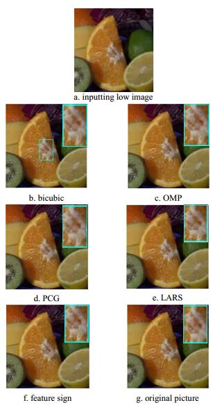
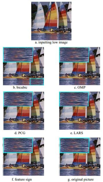
Bicubic reconstructed images are quite fuzzy for lacking of high frequencies while OMP, LARS, and PCG images are short of image details. The edge blur and sawtooth effect are much more obvious in bicubic, OMP, LARS, and PCG, while feature sign pictures are more distinct and clearer. Specifically, as Fig.1 shows, the line of the hat in Lena picture is more fluent and distinct than others in the reconstructed picture. And from the white part of the orange magnified in Fig.2, the proposed method has the clearest picture. Comparing the water ripple in yacht picture, bicubic picture is quite fuzzy, LARS, OMP, PCG pictures have blocking artifact, and the feature sign picture is more discerning.

Table 1 compares the RMSEs of the reconstructed images generated by different methods with different input images. The results show that the proposed algorithm achieves the lowest RMSE against bicubic, LARS, OMP, and PCG. Illustrated by the case of Lena, the RMSE reductions of feature sign over bicubic, LARS, OMP, and PCG are 1.472 1, 0.494 6, 0.480 3, and 0.391 9 respectively.

The reconstruction time of the algorithms is shown in table 2. It can be concluded that the feature sign method yields the best performance with almost the least time. The time of proposed method is nearly one half of LARS and one percent of PCG.

As table 3 presents, the feature sign method can yield the biggest SSIM number, which indicates that the feature sign method can best restore the image. Furthermore, using the feature sign method can improve the efficiency of sparse representation in super resolution.

4.2 Experiment results on a 100-image SR

To test the efficiency of the proposed method more comprehensively, 100 SR experiments are performed by using different algorithms. The 100 test images are downloaded from the international open source image library. The average of RMSE and SSIM are computed in Table 4.

From table 4, the feature sign method yields the lowest RMSE with much less time, also the SSIM value is the biggest, It demonstrates the good quality of the proposed method used in image SR.

5 Conclusion

This paper proposes an efficient sparse representation method called feature sign for single image super-resolution. This method guesses the sign of sparse coefficients, then changes the complicated ${\ell _1}$ -norm question to a QP question. Simulation results demonstrate the advantage of the proposed scheme over existing schemes. Output images from the bicubic have edge blur, OMP pictures have badly jagged artifacts, those from LARS have some blocky effect, and PCG is time wasting, while feature sign reconstructions are distinct and have better visual performance in details. Reconstructed RMSE and SSIM all illustrate the good quality of the proposed method over other methods.