In this section, some basic concepts about algebraic graph theory are firstly introduced. Then we review some notions from non-smooth analysis and differential inclusion. Finally, we formulate the economic dispatch problem of the energy water nexus.

Now we present some notions from algebraic graph theory^[23]. A graph is a triplet ${G = (V;E;{{A}})}$ where V denotes the vertex set, ${E \subseteq V \times V}$ represents the edge set, and ${{A}}$ is the adjacency matrix. An edge from $j$ to $i$ , denoted by ${(i,j)}$ , means that agent $i$ can receive information from agent $j$ . An adjacency matrix is defined by ${{{A}} = [{a_{ij}}] \in {R^{N \times N}}}$ , where ${{a_{ij}} > {\rm{0}}}$ if ${(i,j) \in E}$ and ${{a_{ij}} = {\rm{0}}}$ , otherwise. A graph is undirected if ${(i,j) \in E}$ and ${(j,i) \in E}$ simultaneously. An undirected graph is connected if there is a path between any pair of vertexes. The Laplacian matrix is defined by ${{{L}} = {{D}} - {{A}}}$ , where ${{ D} = {\rm {diag}}\left( {{d_{\rm{1}}},d_{\rm{2}}\cdot \cdot \cdot,{d_N}} \right)}$ with ${d_i} = \displaystyle\sum\limits_{j = 1}^N {{a_{ij}}} $ . For the Laplacian matrix ${{L}}$ , at least one of the eigenvalues of ${{L}}$ is zero and the rest of them have nonnegative real parts. If $G$ is an undirected and connected graph, then $0$ is a simple eigenvalue of ${{L}}$ and the other eigenvalues are positive numbers. Additionally, the eigenvector corresponding to the eigenvalue $0$ is given by ${\upsilon {{{1}}_N}}$ for some constant ${\upsilon }$ . Throughout this paper, the following assumption is used for the graph ${G = (V;E;{{A}})}$ .

Assumption 1: The graph ${G = (V;E;{{A}})}$ is undirected and connected.

We recall some notions from non-smooth analysis^[24]. A function $f:{R^N} \to R$ is locally Lipschitz at ${{{x}} \in {R^N}}$ if there exist positive constants $\varepsilon $ and $\delta $ , such that for any vectors ${{y}},{{z}} \in B({ x},\delta )$ , one has $|f({{y}}) - f({{z}})| \leqslant \varepsilon \left\| {{{y}} - {{z}}} \right\|$ . If $f$ is Lipschitz near any point ${{x}} \in {R^N}$ , then $f$ is said to be locally Lipschitz in ${R^N}$ . If the function $f$ is locally Lipschitz in ${R^N}$ , then $f$ is differential almost everywhere (a.e.) in the sense of Lebesgue measure. The generalized directional derivative of $f$ at ${{x}}$ in the direction ${{v}} \in {R^N}$ is defined,

Furthermore, Clarke’s generalized gradient of $f$ at ${{x}}$ is defined by

If $f:{R^N} \to R$ is a convex function, then one knows that $\partial f({{x}})$ is a nonempty, convex, compact set of ${{R^N}}$ , and $\partial f({{x}})$ is upper semicontinuous at ${{x}}$ .

A time-invariant differential inclusion is given by

where $F$ is a set-valued map from ${{R^q}}$ to the compact convex subsets of ${{R^q}}$ . A solution ${{x}}(t):(0,\tau )\to$ ${R^q}$ for ${\tau > {\rm{0}}}$ of the differential inclusion (1) is an absolutely continuous curve almost everywhere. A set $M$ is said to be weakly invariant (resp., strongly invariant) with respect to (1), if for every ${{{{x}}_{\rm{0}}} \in M}$ , $M$ contains at least a solution (resp., all the solutions) of (1) starting from ${{{x}}_{\rm{0}}}$ . An equilibrium point of (1) is a point ${{{{x}}_e} \in {R^q}}$ with ${{{{0}}_q} \in F({{{x}}_e})}$ . An equilibrium point ${{{z}} \in {R^q}}$ of (1) is Lyapunov stable if, for every ${\varepsilon > {\rm{0}}}$ , there exists ${\delta = \delta (\varepsilon ) > {\rm{0}}}$ such that, for every initial condition ${{{{x}}_{\rm{0}}} = {{x}}({\rm{0}}) \in B({ z};\delta )}$ , every solution ${{{x}}(t) \in B({ z};\delta )}$ for all ${t > {\rm{0}}}$ .

Let ${V{\rm{: }}\,{R^q} \to R}$ be a locally Lipschitz continuous function, and $\partial V$ is the Clarke’s generalized gradient of $V({{x}})$ at ${{x}}$ . The set-valued Lie derivative ${L_F}V:$ ${R^q} \to R$ of $V$ with respect to the differential inclusion (1) is defined by ${L_F}V({ x}) = {\rm{\{ }}a \in R:{{{p}}^{\rm {T}}}{{v}}$ $= a,{{v}} \in F({ x}),$ ${{p}} \in \partial V({ x}){\rm{\} }}$ . In the case when ${{L_F}V({{x}})}$ is nonempty, we use ${{\rm{max}}{L_F}V({ x})}$ to denote the largest element in the set ${{L_F}V({ x})}$ . If $\phi ( \cdot )$ is a solution to (1) and $V:{R^q} \to R$ is locally Lipschitz and regular, then $\dot V(\phi ( \cdot ))$ exists almost everywhere and $\dot V \in {L_F}V(\phi ( \cdot ))$ almost everywhere. In addition, if $V( \cdot )$ is continuous differentiable at ${ x}$ , then ${L_F}V({{x}}) = \{ {{{v}}^{\rm {T}}}\nabla V({{x}}),v \in F({{x}})\}$ . Next, an invariantce principle is presented for non-smooth regular functions^[25].

Lemma 1: For the differential inclusion (1), assume that $F$ is upper semicontinuous and locally bounded, and ${F({{x}})}$ takes nonempty, compact, and convex values. Let ${V{\rm{: }}\,{R^q} \to\, R}$ be a locally Lipschitz and regular function, ${S \subset {R^q}}$ be compact and strongly invariant for (1), $\phi ( \cdot )$ be a solution of (1),

and $M$ be the largest weakly invariant subset of ${{\bar X}} \cap S$ , where ${{\bar X}}$ is the closure of X. If ${\rm{max}}{L_F}V({{x}}) \leqslant 0$ for all ${ x} \in S$ , then $d({{\phi}} (t),M) \to 0$ as $t \to + \infty $ where $d({{\phi}} (t),M) = {\rm{inf}}\{ ||{{\phi}} (t) - {{y}}||,{{y}} \in M\}$ . For scalar $s$ , ${[s]^ + } = s$ if ${s > {\rm{0}}}$ , and ${[s]^ + } = 0$ , otherwise.

We now present a mathematical model for co-optimization of power-water nexus. Let ${{x_{{\rm p}_i}} \in R}$ , ${{x_{{\rm w}_j}} \in R}$ denote the power generated by a power plant $i$ and the water produced by a water plant $j$ , respectively. Let ${{x_{{\rm cp}_k}} \in R}$ and ${{x_{{\rm cw}_k}} \in R}$ denote the power and water produced by a coproduction plant $k$ . Let ${{d_{{\rm p}_i}}}$ , ${{d_{{\rm w}_j}}}$ , ${d_{{\rm cp}_k}}$ and ${d_{{\rm cw}_k}}$ denote the resource product demands of power plant $i$ , water plant $j$ , and coproduction plant $k$ , respectively. The following notations are introduced to vectorize the formulation: ${{{{x}}_{{\rm p}_i}} = {{[{x_{{\rm p}_i}},{\rm{0]}}}^{\rm {T}}}}$ , ${{{{x}}_{{\rm w}_j}} = {{[{\rm{0}},{x_{{\rm w}_j}}]}^{\rm {T}}}}$ , ${{{x}}_{{\rm c}_k}} = {[{x_{{\rm cp}_k}},{x_{{\rm cw}_k}}]^{\rm {T}}}$ , ${{{d}}_{{\rm c}_k}} = {[{d_{{\rm cp}_k}},{d_{{\rm cw}_k}}]^{\rm {T}}}$ , ${{{d}}_{{\rm p}_i}} = {[{d_{{\rm p}_i}},0]^{\rm {T}}},$ ${{{d}}_{{\rm w}_j}} = {[0,{d_{{\rm w}_j}}]^{\rm {T}}}$ . Then the co-optimization problem of power-water nexus is modeled as follows:

where ${f_{{\rm p}_i}}$ , ${f_{{\rm w}_j}}$ and ${f_{{\rm c}_k}}$ are respectively the scalar cost functions for the ith power production facility, the jth water production facility and the kth coproduction facility, ${{N_{\rm{p}}}}$ , ${{N_{\rm{w}}}}$ and ${{N_{\rm{c}}}}$ are the numbers of power, water and coproduction facilities, respectively, and ${{{\underline {{x}} }_{{\rm p}_i}}}$ , ${\underline {{x}} _{{\rm w}_j}}$ , ${\underline {{x}} _{{\rm c}_k}}$ , ${\bar {{x}}_{{\rm p}_i}}$ , ${\bar {{x}}_{{\rm w}_j}}$ and ${\bar {{x}}_{{\rm c}_k}}$ are positive lower and upper bound vectors, respectively.

Remark 1: The equality constraint is a global constraint which denotes the supply-demand balance while the inequality constraints represent the reasonable limits of plants’ production capacity.

Assumption 2: The cost functions ${f_{{\rm p}_i}}$ , ${f_{{\rm w}_j}}$ and ${f_{{\rm c}_k}}$ are convex and continuous differentiable.

Before a distributed algorithm is proposed to solve the optimization problem (2), we need to transform the problem by using the exact penalty function method. We ignore the heterogeneity of the power, water and coproduction plants and define ${{{{{{x}}}}_i} \in {R^{\rm{2}}}}$ as the concatenation vector of ${{{x}}_{{\rm{p}}_i}}$ , ${{{x}}_{{\rm{w}}_j}}$ and ${{{x}}_{{\rm{c}}_k}}$ , thus the index $i$ ranges from 1 to $N = {N_{\rm{p}}} + {N_{\rm{w}}} + {N_{\rm{c}}}$ . Correspondingly, define ${{f_i}({{{x}}_i})}$ as the concatenation vector functions of ${{f_{{\rm{p}}_i}}({{{x}}_{{\rm{p}}_i}})}$ , ${{f_{{\rm{w}}_j}}({{{x}}_{{\rm{w}}_j}})}$ , ${f_{{\rm{c}}_k}}({{{x}}_{{\rm{c}}_k}})$ and ${{{d}}_i}$ as the demand vector. Based on the optimization problem (2), a transformed model is given as follows:

where

and $x_i^j$ , $\underline x _i^j$ and $\bar x_i^j$ denote the jth element of the state variable ${{{x}}_i}$ , the lower bound ${\underline {{x}} _i}$ and the upper bound ${{{\bar x}}_i}$ , respectively. The parameter $\theta $ is a constant and satisfies the following lemma.

Lemma 2 ^[14]: The solutions to the optimization problems (2) and (3) coincide for ${\theta > {\rm{0}}}$ when

where

and the generalized gradient of the function $f_i^\theta $ with respect to the variable $x_i^j$ is given as follows:

Now, a distributed algorithm is provided to solve the problem (3)

where ${{{\lambda}} _i} = {(\lambda _i^{\rm{1}},\lambda _i^{\rm{2}})^{\rm {T}}}$ and ${{{{z}}_i} = {{({{z}}_i^{\rm{1}},{{z}}_i^{\rm{2}})}^{\rm {T}}}}$ for ${i = {\rm{1}}, {\rm{2}},\cdot \cdot \cdot,N}$ . Equivalently, the algorithm (4) can be rewritten as the following vector form,

where ${{{\lambda}} = {{({{\lambda}} _{\rm{1}}^{\rm {T}},{{\lambda}} _{\rm{2}}^{\rm {T}},\cdot \cdot \cdot,{{\lambda}} _N^{\rm {T}})}^{\rm {T}}}}$ , ${{{z}} = {{({{z}}_{\rm{1}}^{\rm {T}},{{z}}_{\rm{2}}^{\rm {T}},\cdot \cdot \cdot,{{z}}_N^{\rm {T}})}^{\rm {T}}}}$ and ${{{d}} = {{({{d}}_{\rm{1}}^{\rm {T}}, {{d}}_{\rm{2}}^{\rm {T}}, \cdot \cdot \cdot,{{d}}_N^{\rm {T}})}^{\rm {T}}}}$ .

Theorem 1: Under assumption 1 and assumption 2, if ${({{{x}}^*},{{{\lambda}} ^*},{{{z}}^*})}$ is an equilibrium point of the distributed algorithm (5), then ${{{{x}}^*}}$ is an optimal solution of the problem (3).

Proof: Since ${({{{x}}^*},{{{\lambda}} ^*},{{{z}}^*})}$ is an equilibrium point of the algorithm (5), then one has,

Because the graph $G$ is undirected and connected, we have ${{{1}}_N^{\rm {T}}{{L}} = {{\textit{0}}}}$ . Furthermore, one has

Thus one has $\displaystyle\sum\limits_{i = 1}^N {{{{x}}_i}} = \displaystyle\sum\limits_{i = 1}^N {{{{d}}_i}}$ . Additionally, since ${({{L}} \otimes {{{I}}_{\rm{2}}}){{{\lambda}} ^*} = {{{0}}_{{\rm{2}}N}}}$ , one has ${{{\lambda}} _{\rm{1}}^* = , {{\lambda}} _{\rm{2}}^* = ,\cdot \cdot \cdot, = {{\lambda}} _N^*}{\rm{ = }}{{\mu}} \in {R^2}$ .

Therefore, the equilibrium point ${({{{x}}^*},{{{\lambda}} ^*},{{{z}}^*})}$ of the algorithm (5) satisfies

which is exactly the optimal condition for problem (3). Thus, the equilibrium point ${{{ x}^*}}$ is the optimal solution of the problem (3). The proof is completed.

Remark 2: From Theorem 1, it is sufficient to show that the algorithm (5) can converge to the optimal solution ${{{{x}}^*}}$ if the algorithm (5) converges to the equilibrium point ${({{{x}}^*},{{{\lambda}} ^*},{{{z}}^*})}$ . Next, we show that the algorithm (5) converges to the equilibrium point.

Theorem 2: For any initial state, the solutions of the algorithm (5) converge to the equilibrium point ${({{{x}}^*},{{{\lambda}} ^*},{{{z}}^*})}$ under assumption 1 and assumption 2.

Proof: Define an energy function

It is noted that there exists a vector ${{{g}} \in \partial {f^\theta }({{x}})}$ such that

for any ${{{g}} \in \partial {f^\theta }({{x}})}$ . Since ${{f^\theta }({{x}})}$ is convex and the Laplacian matrix is positive semidefinite, one has

Thus, ${{\rm{max}}{L_F}V({{x}},{{\lambda}} ,{{z}}) \leqslant {\rm{0}}}$ and $V({{x}}(t),{{\lambda}} (t),{{z}}(t))$ is non-increasing. It is easy to obtain that

Furthermore, the solution ${({{x}}(t),{{\lambda}} (t),{{z}}(t))}$ is bounded. Then we know that

is upper semicontinuous and locally bounded. At the same time, the energy function ${V({{x}},{{\lambda}} ,{{z}})}$ is a locally Lipschitz and regular function. Let $S = {\rm{\{ }}({{x}},{{\lambda}} ,{{z}}):$ $0 \in {L_F}V({{x}},{{\lambda}} ,{{z}}){\rm{\} }}$ . Since ${{L_F}V({{x}},{{\lambda}} ,{{z}}) \leqslant {\rm{0}}}$ , $S$ is a compact and strongly invariant set for the algorithm (5). Thus, according to Lemma 1, the solution of the algorithm (5) starting from any initial value converges to the largest weakly positively invariant set $M$ .

Next, we will show that any solution $({{\bar x}},{{\bar \lambda}} ,{{\bar z}}) \in M$ is an optimal solution of the algorithm (5). Since ${{\rm{0}} \in {L_F}V({{\bar x}},{{\bar \lambda}} ,{{\bar z}})}$ , then one has

Due to ${\left( {{{L}} \otimes {{{I}}_{\rm{2}}}} \right){{{\lambda}} ^*} = {{{0}}_{{\rm{2}}N}}}$ , one has ${\left( {{{L}} \otimes {{{I}}_{\rm{2}}}} \right){{\bar \lambda}} = {{{0}}_{{\rm{2}}N}}}$ . At the same time, it is noted that the Hessian matrix ${{\bf H}({{x}})}$ of the function $f({{x}})$ is positive definite, one has

where ${{\rm{0}} \leqslant \tau \leqslant {\rm{1}}}$ . Hence, we have ${{{\bar x}} = {{{x}}^*}}$ , which implies that ${{\bar x}}$ is an optimal solution of the problem (3). Due to the arbitrariness of $({{\bar x}},{{\bar \lambda}} ,{{\bar z}})$ in $M$ , we can conclude that the equilibrium points in $M$ are all the optimal solutions of the problem (3).

Finally, we prove that the solution ${{x}}(t)$ to the algorithm (5) will converge to the largest weakly positively invariant set $M$ . Define ${{\phi}} (t) = ({{x}}(t),{{\lambda}} (t),$ ${{z}}(t))$ . Since ${\phi (t)}$ is bounded, according to Bolzano-Weierstrass theorem^[26], there exists ${{{\hat \phi}} = ({{\hat x}},{{\hat \lambda}} ,{{\hat z}})}$ and $({t_k},k = {\rm{1,2}}, \cdot \cdot \cdot )$ such that ${{{\phi}} ({t_k}) = ({{x}}({t_k}),{{\lambda}} ({t_k}),}{{z}}({t_k})) \to$ $({{\hat x}},{{\hat \lambda}} ,{{\hat z}})$ as ${k \to + \infty }$ . Since ${{\rm dist}({{\phi}} (t),M) \to {\rm{0}}}$ , then one has ${{{\hat \phi}} \in M}$ and thus ${{\hat x}}$ is an optimal solution of the problem (3). Consider a new Lyapunov function $\bar V({{x}}(t),{{\lambda}} (t),$ ${{z}}(t))$ defined as ${V({{x}}(t),{{\lambda}} (t),{{z}}(t))}$ by replacing $({{{x}}^*},{{{\lambda}} ^*},{{{z}}^*})$ in the equation (6) with ${({{\hat x}},{{\hat \lambda}} ,{{\hat z}})}$ . By similar discussion as above for ${V({{x}},{{\lambda}} ,{{z}})}$ , one has ${{\rm{max}}{L_F}\bar V({{x}},{{\lambda}} ,{{z}}) \leqslant {\rm{0}}}$ . Due to the continuity of $\bar V$ , for any ${\varepsilon > {\rm{0}}}$ , there exists ${\omega > {\rm{0}}}$ such that ${V({{x}},{{\lambda}} ,{{z}}) \leqslant \varepsilon }$ when $||{{\phi}} - {{\hat \phi}} || \leqslant \omega$ . Since $\bar V$ is monotonically non-increasing on the interval $[0, + \infty )$ , there exists a positive integer $T$ such that when ${t \geqslant {t_T}}$ , there is

which implies ${{\rm{li}}{{\rm{m}}_{t \to + \infty }}{{x}}\left( t \right) = {{\hat x}}}$ . Furthermore, since $\bar V$ is radially unbounded with respect to ${{x}}(t)$ , thus the solution ${{x}}(t)$ to the algorithm (5) globally converges to an optimal solution of the problem (3).

Remark 3: It is noted that the algorithm (4) is a differential inclusion and implemented by using only the plant’s neighbors information. The gradient information is not shared in the neighborhood and thus the proposed algorithm can favorably protect the privacy of agents.

In this section, we apply the algorithm (5) to solve the hybrid optimization problem for an energy-water nexus system. It is assumed that the energy-water nexus system consists of 2 power plants, 2 water plants, and 2 coproduction facilities. The communication topology of the system is an undirected and connected graph which is shown in Fig.1. The cost functions ${f_{{\rm p}_i}}$ , ${f_{{\rm w}_j}}$ , ${f_{{\rm c}_k}}$ of the plants are quadratic functions, i.e.,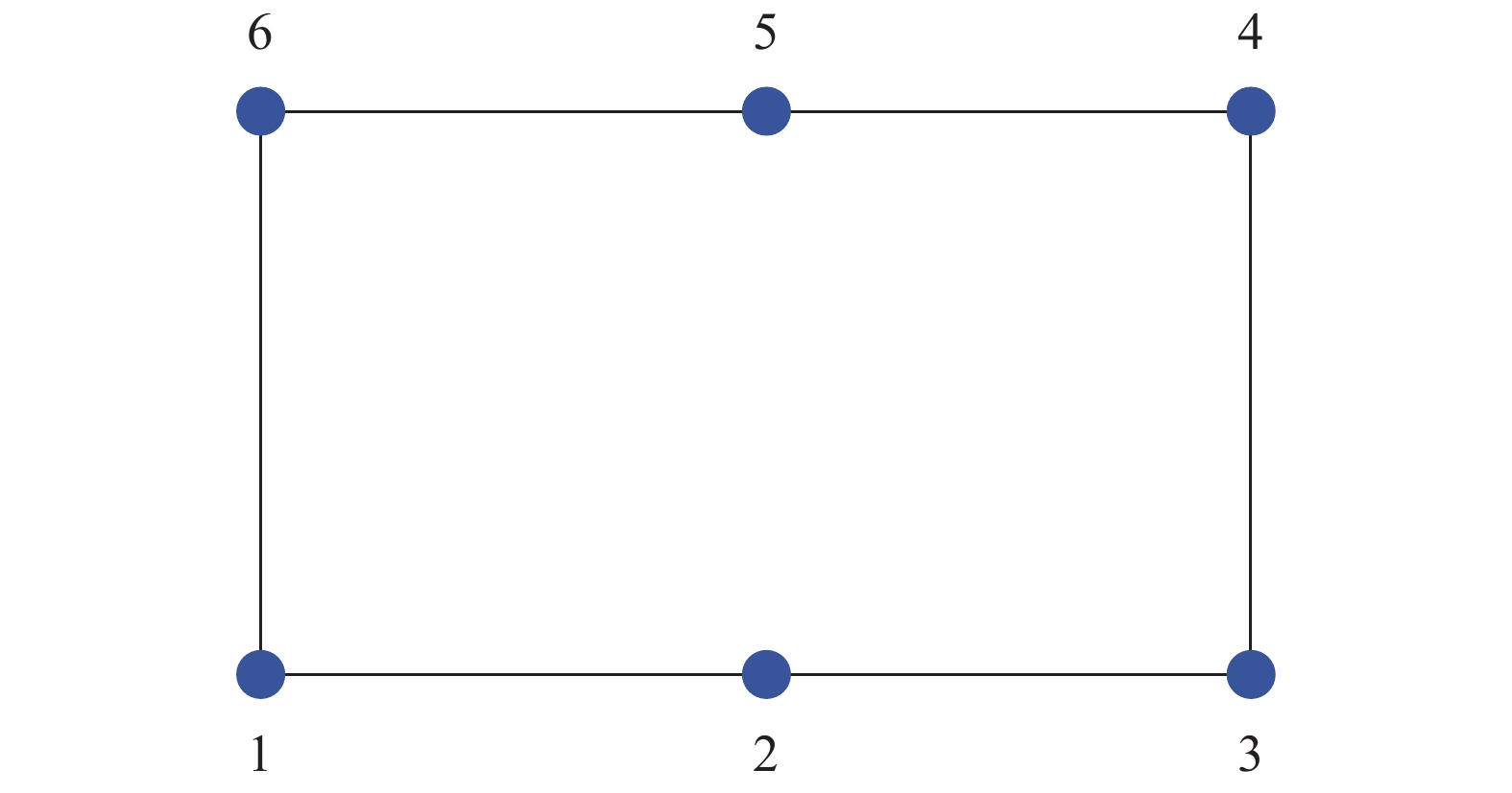

Figure 1.  The communication network

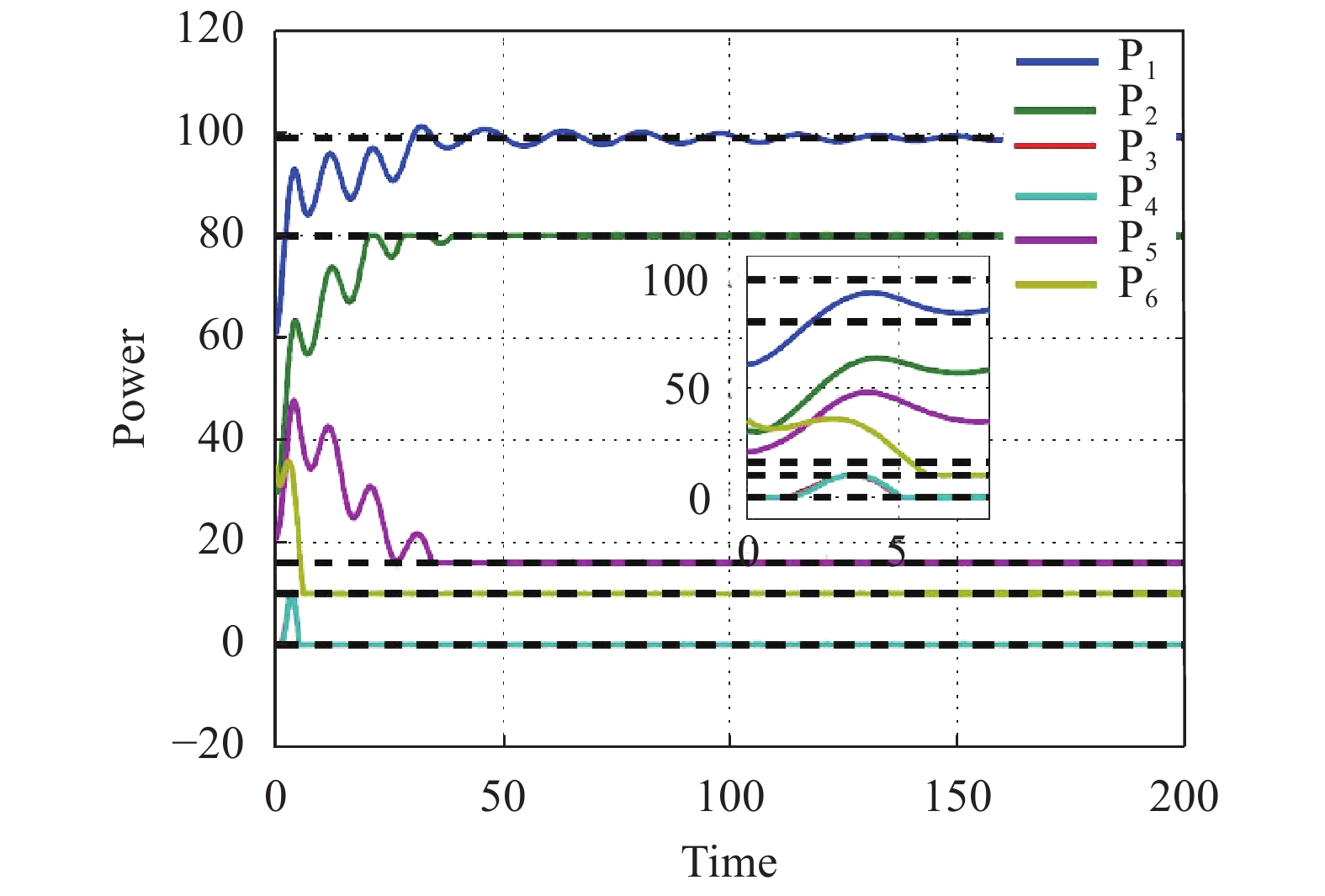
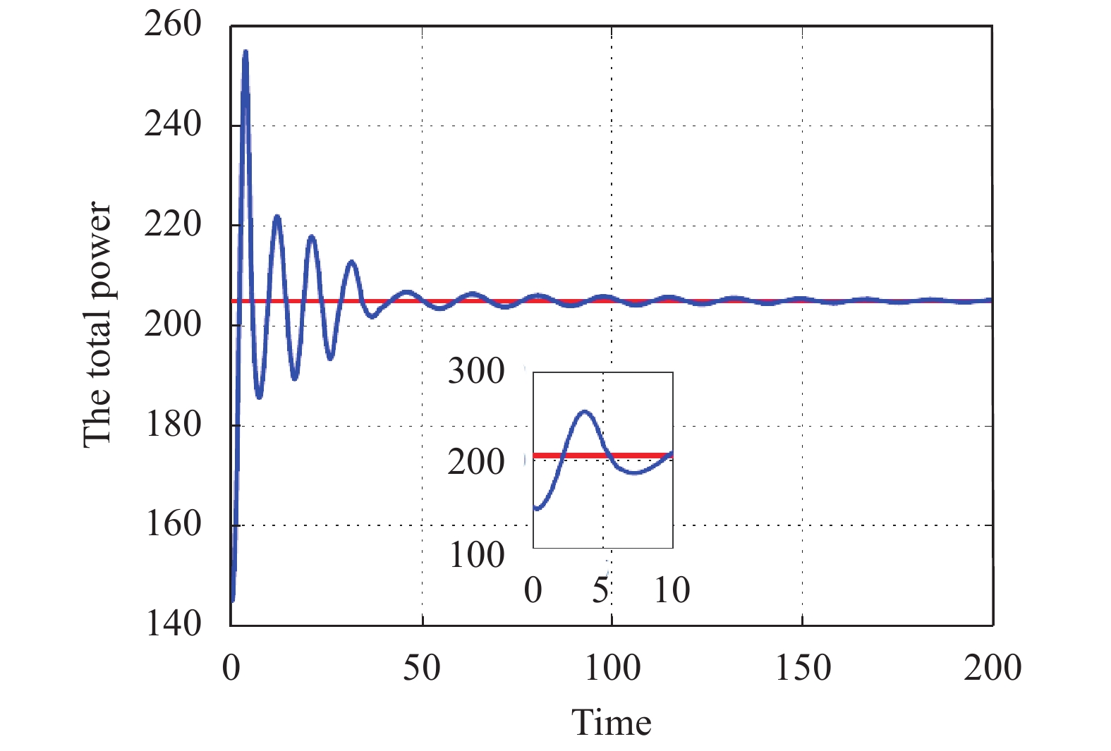
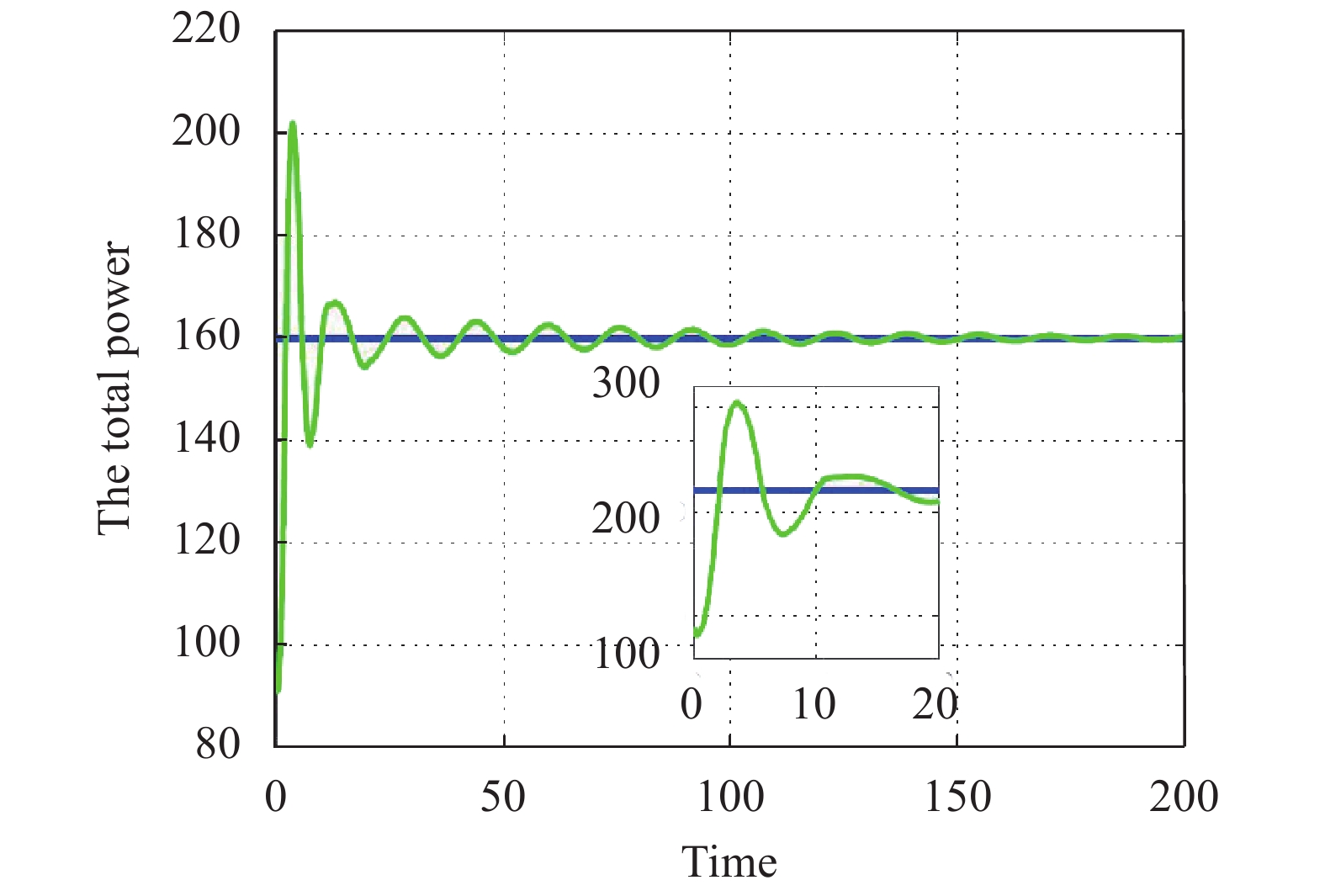
The parameters of the plants are given in Table 1. The demand vector is given by ${{{d}} = [{\rm{90,0}},{\rm{20,0}},{\rm{0,90,0}},{\rm{10,50,20,45,40}}}]^{\rm {T}}$ . The parameter $\theta $ in the penalty function ${{f^\theta }({{x}})}$ is chosen as ${\rm{0}}{\rm{.101\;9}}$ . The initial condition of the algorithm (5) can be randomly given. It is noted that the state ${{{{x}}_i} \in {R^{\rm{2}}}}$ of each agents has two components (i.e., power and water), thus we respectively give the evolution of the power and water states of the six plants under the algorithm (5), as shown in Fig. 2 and Fig. 3. In the figures, the black dashed lines denote the optimal solution of the algorithm (5), which is given by ${{{x}}_{{\rm p}_{\rm{1}}}^* = {\rm{99}}}$ , ${{{x}}_{{\rm p}_{\rm{2}}}^* = {\rm{80}}}$ , ${{{x}}_{{\rm cp}_{\rm{1}}}^* = {\rm{16}}}$ , ${{{x}}_{{\rm cp}_{\rm{2}}}^* = {\rm{10}}}$ for power and ${{{x}}_{{\rm w}_{\rm{1}}}^* = {\rm{50}}}$ , ${{{x}}_{{\rm w}_{\rm{2}}}^* = {\rm{35}}}$ , ${{{x}}_{{\rm cw}_{\rm{1}}}^* = {\rm{40}}}$ , ${{{x}}_{{\rm cw}_{\rm{2}}}^* = {\rm{35}}}$ for water. It can be found that the trajectories of the decision variables about power and water asymptotically converge to the optimal values. Additionally, Fig. 4 and Fig. 5 show that the proposed algorithm can keep the balance of supply and demand of power and water, respectively.

Figure 2.  The evolution of power allocation

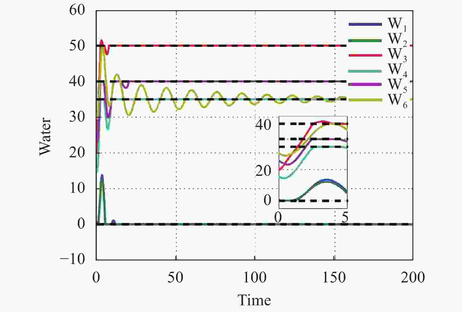
Figure 3.  The evolution of water allocation

Figure 4.  Total mismatch of power

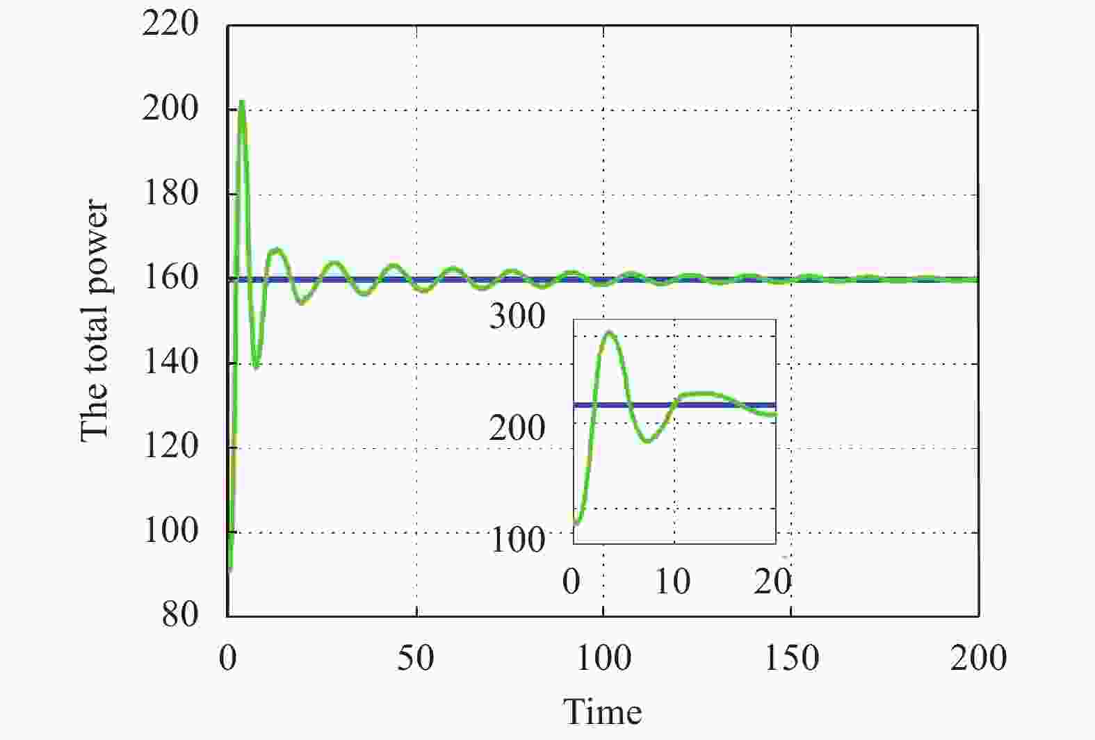
Figure 5.  Total mismatch of water

In this paper, we have designed a distributed continuous-time algorithm which allows a group of power, water, and coproduction plants to solve the economic dispatch problem with local inequality constraints starting from any initial allocation. To accomplish this, we have transformed the original problem by using the exact penalty function method into an equivalent problem without local inequality constraints. Then a distributed algorithm has been proposed to solve the equivalent optimization problem. A theoretical analysis has been presented for the proposed algorithm with the help of algebraic graph theory, Lyapunove function method, and non-smooth analysis. The simulation result indicates that the algorithm is effective and it will save plenty of production cost for the economic dispatch problem of energy-water nexus. In the future, we will further investigate the economic dispatch problem of the energy-water nexus system which not only includes the electricity-storage devices but also the water storage facilities. Moreover, we will consider the power-water production ratio for the coproduction plants in the co-optimization model such that the model is more practical.