ISSN
ISSN 


 下载:
下载:

-
For extracting and analyzing data, we worked out the corresponding software—polar mesosphere echoes and polar mesosphere clouds data extract and analysis software (PMEC_DEAS) that streamlined the analysis processes. PMEC_DEAS compatible with PME_DEAS[1]. Using the software developed, it is possible to analyze data with the range variation of the parameters taken into account. Moreover, much effort has been made to minimize the calculation burden in PMEC_DEAS. In a word, PMEC_DEAS is more versatile, scalable and convenient operation software than other similar type data analysis software.
The paper focuses on the abnormal radar echoes that occur in summer and studies the characteristics of PMSE and PMC. PMC are very thin ice clouds that form near the polar mesopause in the North and South hemispheres. PMC are routinely measured by the lidar technique or satellite[2-6]. Besides, it can be visible to the naked eye possibly after sunset when the lower part of the atmosphere is dark. Therefore, PMC have an interesting and historical name of ‘noctilucent’ (visible during the night) clouds.
PMSE are abnormal strong radar echoes at polar caused by electron density irregularities at half-scale of the radar wavelength for monostatic radars. PMSE were first discovered by Ref.[7]. The occurrence altitude of PMC is lower than that of PMSE. PMC usually occur in the altitude range of 80~86 km[4], while the altitude range of PMSE is relatively wide, in the range of 80~95 km[8]. But it is known from both theoretical and observed results that PMSE are tied up with PMC. Since then, a great deal of researches have focused on the formation mechanism of PMSE and PMC[9-15]. However, the formation mechanism that allows for the keeping of such structures in the ionosphere was a hanging matter for more than forty years. In 2011, Ref.[16] showed that PMC without PMSE mostly occured around midnight and had a great influence on the electromagnetic wave propagation in the mesosphere using the coincident measurements of PMSE and PMC above ALOMAR (69°N, 16°E) by radar and lidar from 1999 to 2008. In 2016, Ref.[17] showed persistent longitudinal variations of PMC in eight years. In fact, changes observed in PMC and PMSE in recent decades are possibly related to anthropogenic effects on the atmosphere. Verification of the relation between PMC and PMSE requires the coincident measurements equipment while observing PMC and PMSE.
In the paper, the data of PMSE and PMC are analyzed by PMEC_DEAS. We presented the correlation between short-term coincident measurements PMSE and PMC above Tromsø on 13-15 July 2010, 24-28 June 2013 and 1 July 2013, respectively. The correlation between long-term coincident measurements of PMSE and PMC during 2007-2013 is also analyzed. It is one of the few studies for long-term analysis on the correlation between the PMSE and PMC. Moreover, the possible explanations are discussed.
-
We know that beamforming is a process of combining the individual receive channels into a single received signal. The beamforming can be seen as a spatial filter applied in different complex weights of channels. Some of the results effectively steer a beam in a specific direction. Beamforming gives information about the bearing elevation of the object that users are trying to track. Traditionally, the concept of range-gates is the basis of incoherent scatter signal analysis, in which an assumption is made, that is, the slow spatial change of the target is assumed as a function of the scattering point[18]. PMEC_DEAS is able to analyze radar data and non-radar data. Note that, the raw data should be preprocessed by the GUISDAP (Grand Unified Incoherent Scatter Design and Analysis Package), if the raw data are downloaded from European Incoherent Scatter (EISCAT) dataset website. If not, users can analyze the data by PMEC_DEAS directly. Therefore, PMEC_DEAS has the following purposes:
1) It quickly obtains the dada with processing easily.
2) It completes high-resolution figures of abnormal radar echoes and clouds at the polar mesosphere.
3) It quickly analyzes the variation trends of plasma parameters under changing background environments at the polar mesosphere.
The framework of PMEC_DEAS is easy enough for anyone to participate in, without requiring any understanding of its advanced features. And the user interface (UI) has simple operation, ease and common calibration. However, the following are needed: 1) A computer with MATLAB license; 2) An initialization file for the experiment; 3) The raw data have dealt with by the GUISDAP, if the raw data are downloaded from the EISCAT website; 4) A startup program for the analysis. In short, PMEC_DEAS is mainly divided into four modules:
1) File selection module
The file selection module is the first startup program of the PMEC_DEAS. The purpose of this program is to display the file location and guide the users to select the data to be processed. It makes the selection of data more intuitive and convenient. After reading the data, the data are stored in the form of global variables while transferred to the next program. The module is mainly realized by the ‘uigetfile’ in the MATLAB function library. Fig. 1 shows the graphical interface of the PMEC_DEAS.

Figure 1. Graphical interface of the PMEC_DEAS
2) Data extraction module
The goal of the data extraction module is to extract the data and store them in a ‘.txt’ file, which can extract a variety of data parameters. These data are used by subsequent programs.
3) Data analysis module
The aim of the data analysis module is to perform a preliminary fitting of the extracted data and obtain elementary information. The information includes the figures/profiles of the abnormal echoes and clouds change with the altitude and time at the polar mesosphere.
4) General-purpose graphics module
This module is divided into five sections because users need to extract a variety of effective information from the data. General-purpose graphics module includes the analysis results dominated by the conventional ‘manda’ and ‘arc_dlayer’ mode, analysis results dominated by aspect sensitivity, analysis results dominated by HF heating, and analysis results dominated by the characters of PMC. The characters of abnormal radar echoes can be quickly obtained using conventional ‘manda’ and ‘arc_dlayer’ modes. Users can get the changes with altitude and time of the abnormal radar echoes at the polar mesosphere when the abnormal radar echoes are heated by a powerful ground-based HF radio wave, using the HF heating mode. Besides, the scattering characteristics of the abnormal echoes at the polar mesosphere observed at different elevation angles are obtained, using the aspect sensitivity mode. The section of PMC presents the variations of PMC with different latitudes and longitudes, and users freely choose the PMC data of geographic location which they need.
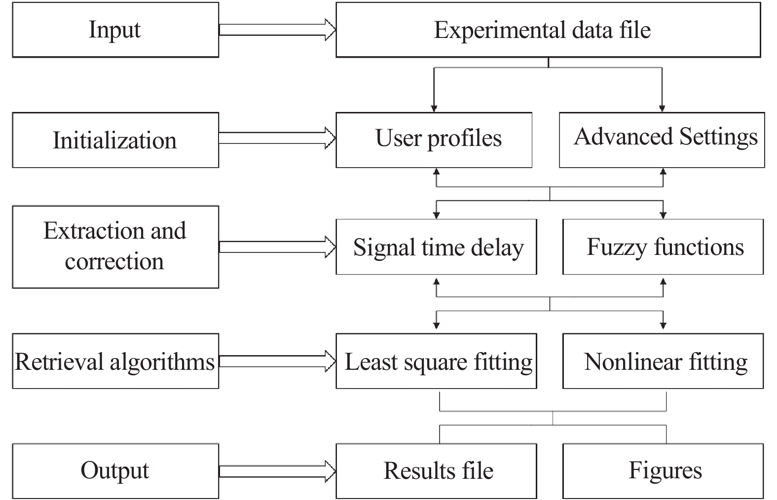
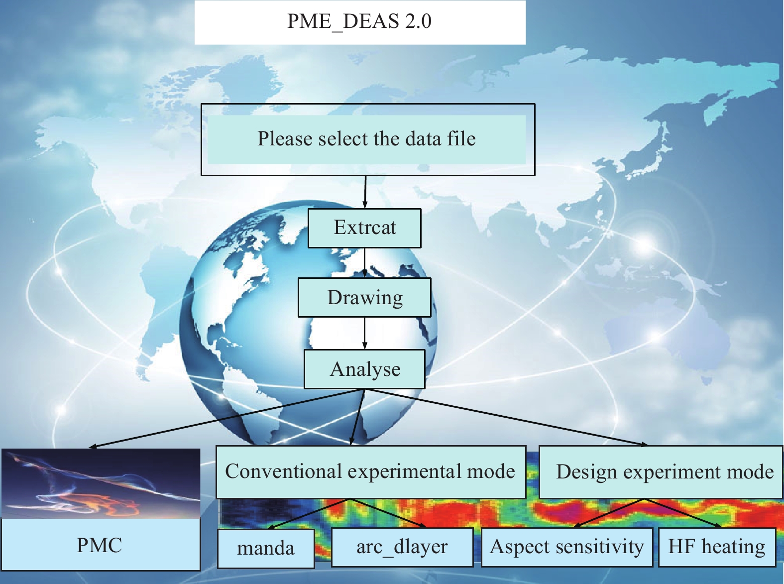
In general, PMEC_DEAS provides a friendly interface to quickly extract the data from a database. During data analysis, users can invoke data in the database, complete high-precision drawing, and obtain an overall understanding of the results of observation experiments. PMEC_DEAS also quickly gives the radar echoes intensity figures in different altitude ranges. Besides, the maximum, average and median values of plasma parameters over time and radar elevation angles are obtained, which are used to study the characteristic of volume reflectivity dependence on the frequency and aspect sensitivity of radar echoes and other characteristics. At the same time, the influence of HF electromagnetic waves on the plasma is also analyzed in the mesosphere. Moreover, the characters of PMC are also given. Fig. 2 shows the flowchart of the PMEC_DEAS.
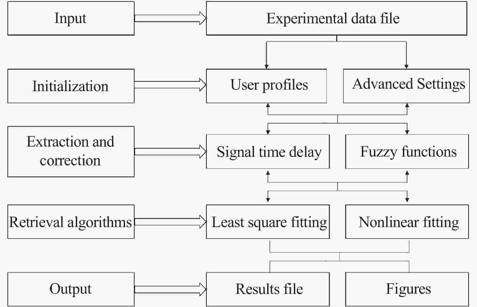
Figure 2. Flowchart of the PMEC_DEAS
-
We analyze the PMSE and PMC dataset by the PMEC_DEAS, then the short-term and long-term correlations between PMSE and PMC are studied as an example in this section. For short-term analysis, the data were collected on 13-15 July 2010, 24-28 June 2013 and 1 July 2013, using EISCAT VHF radar and Cloud Imaging and Particle Size (CIPS) instrument at Tromsø (69°35′N, 19°14′N). For long-term analysis, we use the data collected in 2007-2013.
-
As described above, PMC are observed by the CIPS instrument and PMSE are observed by the EISCAT VHF radar at Tromsø.
-
The EISCAT VHF radar operates at 224 MHz and has a 120 m×40 m parabolic cylinder antenna. The radar working mode—arc_dlayer is used in our study. The PMSE data with altitude resolution of 300 m and time resolution 5 s obtained by the radar are used. The background noise of cosmic origin is removed from the echoes. Additionally, typical contaminations of radar echoes measurements like meteor echoes are removed from the dataset. The details of the technical parameters/modes configuration of the EISCAT VHF radar please refer to Ref. [19] and references therein.
-
The CIPS instrument is a panoramic imager that measures ultraviolet radiation scattered by PMC and atmospheric gases, and it was carried by the NASA Aeronomy of Ice in the Mesosphere (AIM) in 2007[20-21]. The data of CIPS are freely available and updated for each subsequent season (please visit the website: http://aim.hamptonu.edu). The instrument performance requirements for all of the CIPS measurements and the key performance characteristics of the cameras are shown in Table 1[21] and Table 2[21], respectively.
Table 1. CIPS performance requirements configuration[21]
Geophysical parameter resolution Accuracy/% PMC detection limit 50 N/A PMC morphology 50 15 PMC particle size 200 50 Gravity wave effects 3 N/A Table 2. CIPS instrument configuration[21]
Parameter Value Effective focal length/mm 24.8 Focal ratio F/4 Field of view/(°) 44×44 Spectral passband/nm 265±7.5 Pixel size/mm 0.014 Imaging pixel format 2048×2048 According to the measured albedo, the structure of PMC[22] and gravity waves (GWs)[23] can be derived. CIPS PMC data products include cloud albedo, particle radius and ice water content along each orbit strip with 56.25 km2 spatial resolution[22]. In the dataset, the variables that the users are interested in the CLD_ALBEDO (the column integrated brightness "as seen from above") and possibly PARTICLE_RADIUS. As a start, the one CIPS pixel can be found that are closest in latitude and longitude to Tromsø, and then grab the pixels in a square of roughly 30 pixels×30 pixels around this closest pixel. Since one pixel has a size of 7.5 km, it would mean the pixels in a square of 225 km×225 km above the VHF radar. Then do an average over these pixels for each day.
-
The correlation between PMSE observed by the EISCAT VHF radar on 13-15 July 2010, 24-28 June and 1 July 2013 and PMC observed by the CIPS instrument in simultaneous and common-volume observations are studied.
-
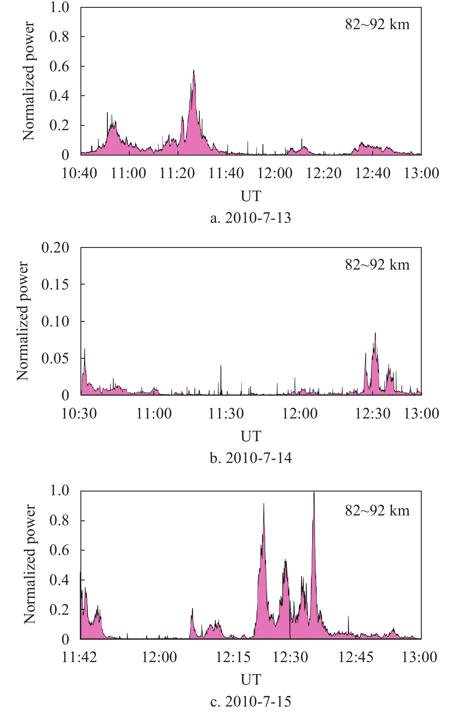
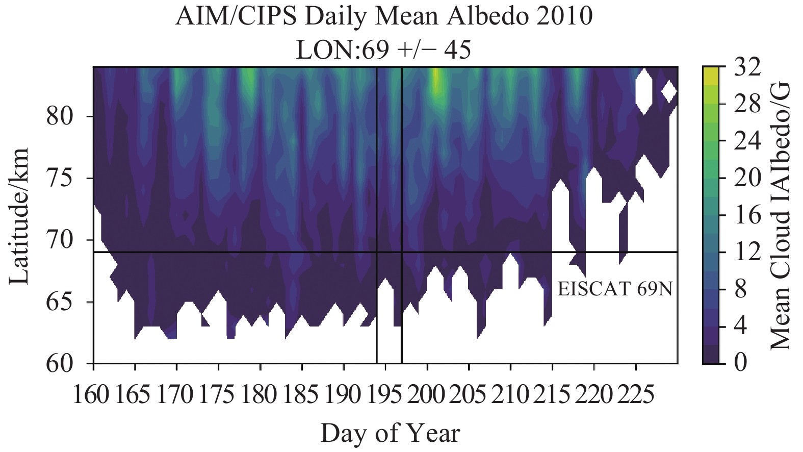
Fig. 3 shows profiles of PMSE normalized intensity on 13-15 July 2010 where the vertical axis shows the average PMSE power during the altitude range of 82~92 km. Fig. 4 shows a profile of PMC intensity in June and July of 2010 where two black lines represent the special latitude (horizontal line) and the timeline (vertical line) corresponding to the observation time of PMSE. It can be seen from Fig. 3 that the strongest radar echo occurred on 15th July 2010, followed by the 13th July, and the weakest radar echo occurred on the 14th July. Besides, it can be noted that the PMC intensity compared with PMSE intensity over Tromsø was relatively weak on 13-15 July 2010, but the PMC intensity on the 15th July was higher than that on 13th and 14th July. This implies that the variational trends of PMSE are consistent with the variational trends of PMC during the observation experiments (13-15 July 2010).

Figure 3. PMSE intensity profile on 13-15 July 2010
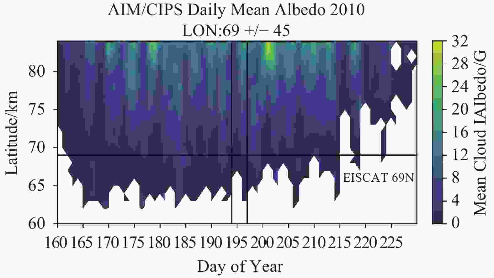
Figure 4. PMC intensity profile on June and July 2010
-
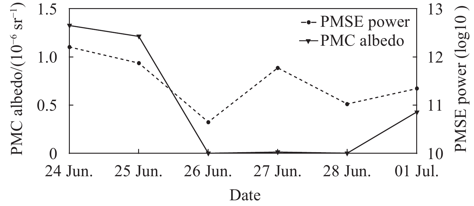
In order to verify the correlation between the short-term PMSE and PMC obtained from section 2.2.1, the correlation between PMSE and PMC is conducted again, using the data from 24-28 June and 1 July 2013. It is necessary to elaborate on the discontinuity of the data. PMSE is only observed on 24-28 June and 1 July by the EISCAT VHF radar in the summer of 2013, so we use the 6 days observational data to analyze the short-term PMSE. The correlation between PMC and PMSE is shown in Fig. 5. The Fig. 5 indicates that the variational trends of PMC and PMSE are generally consistent during 24-28 June and 1 July 2013. Subsequently, we calculate the correlation coefficient between PMC and PMSE. The correlation coefficient is R=0.870, where P=0.046. It suggests that there is a strong positive correlation between PMC and PMSE during 24-28 June and 1 July 2013. Here PMC is positively correlated to the PMSE intensity, indicating that a large fraction of these cases are due to the variation of electron density. Quantification of the relation between PMSE and PMC, especially the short-term observations of PMC and PMSE in the same volume, is beneficial to test PMSE theories and comparison of the boundaries of both phenomena allows to access the strength of the coupling of the layers.
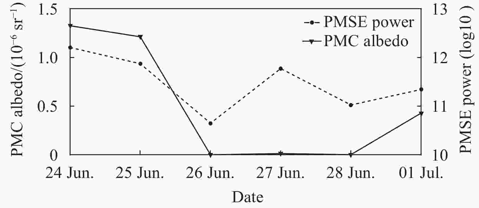
Figure 5. Corresponding PMC and PMSE intensity on 24-28 June and 1 July 2013
-
In section 2.2, we study the short-term correlation between PMSE and PMC, and the long-term correlation between PMSE and PMC is studied in this section. Since CIPS has performed PMC observation missions since 2007, based on our knowledge and published references [16, 24-25], the correlation between PMC and double-layer PMSE might be relatively stronger. Therefore, the correlation between double-layer PMSE and PMC is discussed. Here, for avoiding the impacts of other factors on the correlation, we analyze the PMSE and PMC data during 2007-2013, because there was no apparent PMC when PMSE occurred in 2014 and the following few years. It should be noted that the past data rarely affected the long-term trend in general, and the results of PMSE and PMC described in the paper are relevant for the interpretation and planning now underway.
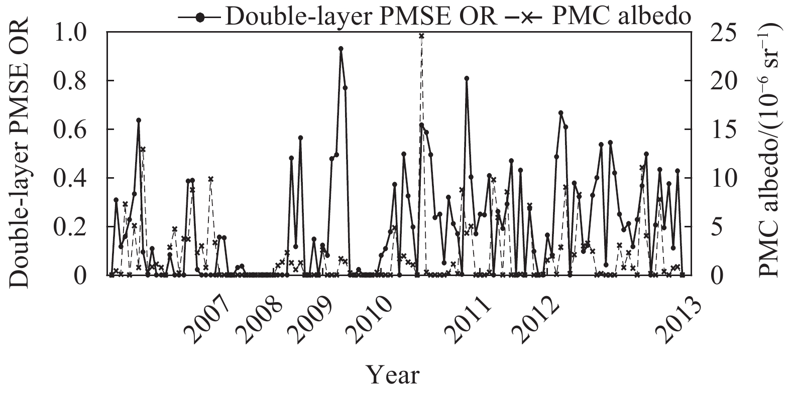
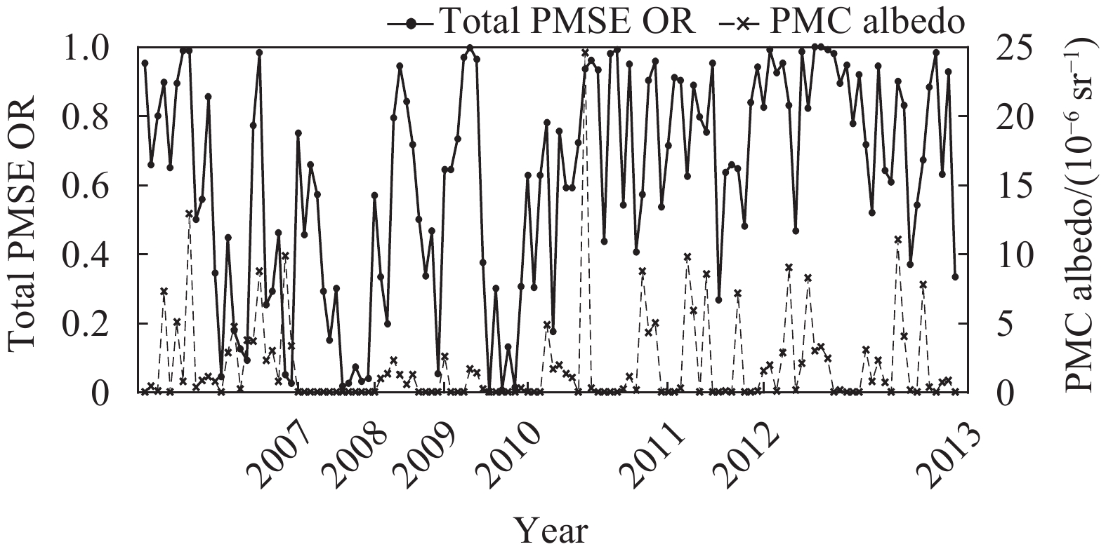
The PMC data are statistically analyzed corresponding to the occurrence of PMSE and the Pearson correlation method (For a detailed introduction of the Pearson correlation method please refer to Ref.[19] and Ref.[26] and references therein) is used to calculate the correlation coefficient between them. If PMSE occur on a certain day, PMC are not observed, then the PMC intensity on that day is recorded as 0. Fig. 6 shows the correlation between the double-layer PMSE occurrence rate (OR) and PMC intensity during 2007-2013. The Pearson correlation coefficient between the double-layer PMSE and PMC is calculated. The correlation coefficient is R= 0.233, where P=0.008. From the perspective of the correlation coefficient, it can be noted that there is a weak correlation between the double-layer PMSE and PMC. Fig. 7 shows the comparative analysis between the total OR of PMSE and the intensity of PMC from 2007 to 2013. The Pearson correlation coefficient between the total PMSE OR and PMC is 0.214 with P=0.005. Therefore, as noted above, the correlation between total PMSE OR and PMC is weak or even irrelevant. But the OR of PMSE is higher than the PMC. In the above analysis process, we notice that there is a situation where at least one of the double-layer PMSE OR or PMC is 0, and the existence of this situation affects the result of correlation. Hence, we should avoid the situation.

Figure 6. Occurrence rate of double-layer PMSE and PMC during 2007-2013

Figure 7. Occurrence rate of total PMSE and PMC during 2007-2013
Avoiding the situation that one of the double-layer PMSE OR or PMC is 0 means that in the process of data analysis, the PMSE OR and PMC intensity data of that day are discarded when one of the double-layer PMSE OR or PMC intensity on a certain day is 0. The data for that day will be retained and the values are both recorded 0, when the PMSE OR and PMC intensity are both 0. Fig. 8 depicts the comparison between the OR of double-layer PMSE and PMC after avoiding the situation that one of the double-layer PMSE OR or PMC is 0 during 2007-2013. It is worth noting that there are still a few PMC intensities seem to equal zero in Fig. 8, in fact, the intensity is not zero, just very weak. After removing the case where one of the double-layer PMSE OR or PMC is 0, the correlation coefficient between them is calculated. The result is correlation coefficient R=0.397, where P=0.042. It is noted that the value of the correlation coefficient between the double-layer PMSE OR and PMC increases compared with that in Fig. 6, showing a moderate correlation. This is in accordance with the results of the previous study[16]. We take this as an indication that the intensities of PMC and PMSE increase due to an increase in electron density in general. Additionally, small-scale structures in ice layers as known from visual observations and ice layers tilts as known from the measurements of PMC also cause uncertainty. As mentioned above, the formation and development of PMSE and PMC are affected by many complex factors. For example, the PMSE and PMC are links to the winds in the mesopause region, and in particular with the meridional winds. The analyses and researches provide new ideas for the research on the formation mechanism of PMSE and PMC. It's reasonable to expect that it will enhance the flexibility of signal processing and promote the development of radar communication system.
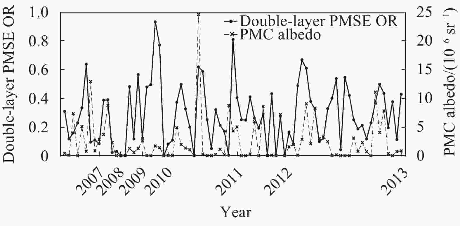
Figure 8. Occurrence rate of double-layer PMSE and PMC during 2007-2013 without both zero at the same time
-
The occurrence of PMC or PMSE is an indicator that the temperature is below the ice point. For example, PMC provide indirect information to measure temperature in regions of the atmosphere where data are lacking. Besides, the PMC observed by lidar are mainly ice particles with a diameter of about tens of nanometers, while PMSE observed by radar indicate the existence of ice particles of different sizes, so smaller ice particles may form at the mesopause and then begin to precipitate. The distribution of electrons may change due to those ice particles, resulting in the variation and inhomogeneous distribution of electron density. The generated ionospheric electron density inhomogeneity will cause the refraction and scattering of radio waves when PMSE and PMC occur. As a result, the radio wave communication between the satellite and the ground is interrupted, and the accuracy of target localization is reduced, and the monitoring and tracking systems of spacecraft (satellites and missiles) fail. There has a serious impact on satellite operation and control, radio communications, global positioning systems and navigation, and space-to-ground monitoring. Therefore, understanding the variation trend of PMSE and its influence on PMC aid in the research of finding one new way to derive the effect of HF electromagnetic waves travelling through the ionosphere and provide a guarantee for the further development of radar communication technology. In principle, the vertical structure of PMC can change with the changes of background atmosphere (e.g. temperature, water vapour content and other dynamic processes)[27]. PMSE and PMC both have temporal-spatial characters, that is, their characters change with time and space. Nonetheless, Ref.[9] first reported the coincidence of PMSE and PMC bottom altitudes from different locations. In 2004, Lübken et al. found the coincidence of PMSE and PMC bottom altitudes in Spitsbergen[11]. In 2008, Klekociuk et al. showed that the PMSE and PMC bottom altitudes are coincided in Antarctica[24]. Thus, there are some common factors or interaction fueling the formation of PMSE and PMC. Moreover, In 2011, Kaifler et al. indicated that ice particles are only a necessary but not a sufficient condition for PMSE formation[16]. These imply that ionization and turbulent activity are necessary conditions, but they might be limited especially at low altitudes. There may be a very rapid sublimation due to the PMSE is sensitive to a wider spectrum of ice particle sizes.
The PMSE have layered structures in mesopause, so do the PMC. In 2012, a few double-layer structures and periodic enhancements in brightness in PMC were observed by Ref.[28], presented multi-layer structure and waves in PMC using the ALOMAR lidar[29]. This implies that PMSE and PMC are similar in the structures and different in the formation mechanism. View from the current study, the formation of layered PMC might due to two or more kinds of different cloud systems across the vertical wind shear region. The possible mechanism of PMSE might be that there is a layered dust particle layer or ice particles, which causes the inhomogeneous distribution of electron density. Therefore, the reflection, refraction and other events of electromagnetic wave transmission in this complex medium are changed. In the plasma, the changes caused by high-power radio waves can affect the transmission of other radio waves in the current region. And as mentioned above, there are interactions between special phenomena (PMSE, PMC and other phenomena) in the ionosphere, which will affect the long-distance communication of electromagnetic waves in the ionosphere. However, the formation processes of PMC and PMSE are still intriguing and open issues. The issue is one of the most important scientific problems, and it needs more attention. Luckily the formation processes of PMSE and PMC can be used to monitor the dynamic processes that lead to their existence. If so, we have reason to believe that the new progress will achieve quickly.
-
A new radar data analysis software is given, and in the examples of this paper, we analyze the PMSE experiment data observed by 224 MHz EISCAT VHF radar and PMC data observed by CIPS from the same geographical location by using PMEC_DAES. The short-term correlation between PMSE and PMC on 13-15 July 2010 and 24-28 June 2013 and 1 July 2013 are presented, respectively. Moreover, the long-term correlation between PMSE and PMC during 2007-2013 is analyzed. By analyzing the PMSE and PMC data on 13-15 July 2010, it can be seen that the PMC intensity on the 15th July is greater than the PMC intensity on the 13th July and 14th July, and there is a positive correlation between the PMSE and PMC during the observation experiment period (24-28 June and 1 July 2013). In addition, the correlation between the PMSE OR and PMC is also statistically analyzed based on the PMC and PMSE data from 2007 to 2013. It is found that the OR of PMSE is higher than that of PMC. But the correlation between the double-layer PMSE OR and PMC is not significant during 2007-2013. After removing the case where one of the double-layer PMSE OR or PMC is 0, it is found that the double-layer PMSE OR and PMC have a moderately positive correlation. It shows that the formation and development of double-layer PMSE are closely related to PMC, which provides favourable support for the theory of PMSE partial formation, and also provides new ideas for solving the issue of radar signal processing when there is PMSE or PMC. Hence, PMEC_DEAS is certainly practical software for analyzing a large dataset. Last but not least, the future development of the software will include more general function models for parameters beyond the existing calculation models in PMEC_DEAS.
-
We are grateful to the EISCAT Scientific Association, China Research Institute of Radiowave Propagation (CRIRP) and the University of Colorado Boulder for providing the PMSE and PMC experimental data. We thank Abdel Hannachi and Lina Broman of Stockholm University for their help in explaining the variables of PMC data. The EISCAT Scientific Association is supported by China (China Research Institute of Radiowave Propagation), Finland (Suomen Akatemia of Finland), Japan (the National Institute of Polar Research of Japan and Institute for Space-Earth Environmental Research at Nagoya University), Norway (Norges Forkningsrad of Norway), Sweden (the Swedish Research Council), and UK (the Natural Environment Research Council).
-
The data that support the findings of this study are openly available in Madrigal Database at EISCAT and LASP’s Data Systems, which were downloaded from https://www.eiscat.se/schedule/schedule.cgi and http://aim.hamptonu.edu.
Study on the Strong Radar Echoes at Polar Mesosphere Using a New Dataset Analysis Software
-
摘要: 该文利用极区中层异常回波及云粒子数据提取分析软件(PMEC_DEAS)处理雷达回波及云粒子数据集,并进行回波特性研究。以通过PMEC_DEAS分析的短期和长期极地中层夏季回波(polar mesosphere summer echoes, PMSE)和极地中层云(polar mesospheric clouds, PMC)数据为例,研究了PMSE出现率与PMC之间的相关性。研究发现短期的PMSE出现率和PMC之间的相关性不显著,长期的双层PMSE出现率与PMC之间呈正相关关系。这表明双层PMSE与PMC密切相关,这与现有的结论一致。以此可以看出,PMEC_DEAS可以有效地适应所研究事件的复杂特征变化,并具有良好的鲁棒性。此外,利用PMEC_DEAS软件分析所得的数据具有更好的稳定性和兼容性,与目前的主流数据分析软件相比更具便捷性和实用性。Abstract: Polar mesosphere echoes and polar mesosphere clouds data extraction and analysis software (PMEC_DEAS) is used to deal with the echoes and clouds dataset, then the characteristics of radar echoes are studied in the paper. By analyzing the polar mesosphere summer echoes (PMSE) and polar mesospheric clouds (PMC) data in the short-and long-terms as an example based on the PMEC_DEAS, the correlation between the occurrence rate (OR) of PMSE and PMC is studied. It is found that the correlation between the short-term PMSE OR and PMC is not significant, the long-term double-layer PMSE OR is positively correlated with the PMC. It shows that double-layer PMSE is closely related to PMC, which is consistent with existing conclusions. PMEC_DEAS can effectively adapt to the complex characteristic changes of the events and has good robustness. The data analyzed by PMEC_DEAS exhibit better stability and compatibility, and show superiority in convenience and utilitarian nature over the current mainstream software.
-
Key words:
- PMEC_DEAS /
- polar mesospheric clouds /
- polar mesosphere summer echoes /
- robustness
-
Figure 8. Occurrence rate of double-layer PMSE and PMC during 2007-2013 without both zero at the same time
-
[1] [2] LESLIE R. The sky-glows[J]. Nature, 1884, 30(781): 583. doi: 10.1038/030583a0 [3] THURAIRAJAH B, CULLENS C Y, BAILEY S M. Characteristics of a mesospheric front observed in polar mesospheric cloud fields[J]. Journal of Atmospheric and Solar-Terrestrial Physics, 2021(218): 105627. [4] GERDING M, KOPP M, HOFFMANN P, et al. Diurnal variations of midlatitude NLC parameters observed by daylight-capable lidar and their relation to ambient parameters[J]. Geophysical Research Letters, 2013, 40(24): 6390-6394. doi: 10.1002/2013GL057955 [5] DUFT D, NACHBAR M, LEISNER T. Unravelling the microphysics of polar mesospheric cloud formation[J]. Atmospheric Chemistry and Physics, 2019, 19(5): 2871-2879. doi: 10.5194/acp-19-2871-2019 [6] HERVIG M E, STEVENS M H, GORDLEY L L, et al. Relationships between polar mesospheric clouds, temperature, and water vapor from solar occultation for ice experiment (SOFIE) observations[J]. Journal of Geophysical Research: Atmospheres, 2009, 114(D20203): 1-11. [7] CZECHOWSKY P, RÜSTER R, SCHMIDT G. Variations of mesospheric structures in different seasons[J]. Geophysical Research Letters, 1979, 6(6): 459-462. doi: 10.1029/GL006i006p00459 [8] LATTECK R, BREMER J. Long-term variations of polar mesospheric summer echoes observed at Andya (69°N)[J]. Journal of Atmospheric and Solar-Terrestrial Physics, 2017, 163(3): 31-37. [9] VON Z U, BREMER J. Simultaneous and common-volume observations of noctilucent clouds and polar mesosphere summer echoes[J]. Geophysical Research Letters, 1999, 26(11): 1521-1524. doi: 10.1029/1999GL900206 [10] KIRKWOOD S, CHO J, HALL C M, et al. A comparison of PMSE and other ground-based observations during the NLC-91 campaign[J]. Journal of Atmospheric and Terrestrial Physics, 1995, 57(1): 35-44. doi: 10.1016/0021-9169(93)E0032-5 [11] LÜBKEN F J, ZECHA M, HÖFFNER J, et al. Temperatures, polar mesosphere summer echoes, and noctilucent clouds over Spitsbergen (78o N)[J]. Journal of Geophysical Research: Atmospheres, 2004, 109(D11203): 1-14. [12] TAYLOR M J, ZHAO Y, PAUTET P D, et al. Coordinated optical and radar image measurements of noctilucent clouds and polar mesospheric summer echoes[J]. Journal of Atmospheric and Solar-Terrestrial Physics, 2009, 71(6): 675-687. [13] GE S C, LI H L, MENG L, et al. On the radar frequency dependence of polar mesosphere summer echoes[J]. Earth and Planetary Physics, 2020, 4(6): 571-578. [14] URCO J M, CHAU J L, WEBER T, et al. Enhancing the spatiotemporal features of polar mesosphere summer echoes using coherent MIMO and radar imaging at MAARSY[J]. Atmospheric Measurement Techniques, 2019, 12(2): 955-969. doi: 10.5194/amt-12-955-2019 [15] LATTECK R, RENKWITZ T, CHAU J L. Two decades of long-term observations of polar mesospheric echoes at 69°N[J]. Journal of Atmospheric and Solar-Terrestrial Physics, 2021(216): 105576. [16] KAIFLER N, BAUMGARTEN G, FIEDLER J, et al. Coincident measurements of PMSE and NLC above ALOMAR (69°N, 16°E) by radar and lidar from 1999-2008[J]. Atmospheric Chemistry and Physics, 2011, 11(10): 1355-1366. [17] LIU X, YUE J, XU J Y, et al. Persistent longitudinal variations in 8 years of CIPS/AIM polar mesospheric clouds[J]. Journal of Geophysical Research: Atmospheres, 2016, 121(14): 8390-8409. doi: 10.1002/2015JD024624 [18] LEHTINEN M S, HUUSKONEN A, PIRTTILÄ J. First experiences of full-profile analysis with GUISDAP[J]. Annales Geophysicae, 1996, 14(12): 1487-1495. doi: 10.1007/s00585-996-1487-3 [19] GE S C, LI H L, XU T, et al. Characteristics of the layered polar mesosphere summer echoes occurrence ratio observed by EISCAT VHF 224 MHz radar[J]. Annales Geophysicae, 2019, 37(3): 417-427. doi: 10.5194/angeo-37-417-2019 [20] HOFFMANN P, RAPP M, FIEDLER J, et al. Influence of tides and gravity waves on layering processes in the polar summer mesopause region[J]. Annales Geophysicae, 2008, 26(12): 4013-4022. doi: 10.5194/angeo-26-4013-2008 [21] MCCLINTOCK W E, RUSCH D W, THOMAS G E, et al. The cloud imaging and particle size experiment on the Aeronomy of Ice in the mesosphere mission: Instrument concept, design, calibration, and on-orbit performance[J]. Journal of Atmospheric and Solar-Terrestrial Physics, 2009, 71(3): 340-355. [22] LUMPE J D, BAILEY S M, CARSTENS J N, et al. Retrieval of polar mesospheric cloud properties from CIPS: Algorithm description, error analysis and cloud detection sensitivity[J]. Journal of Atmospheric and Solar-Terrestrial Physics, 2013(104): 167-196. [23] RANDALL C E, CARSTENS J, FRANCE J A, et al. New AIM/CIPS global observations of gravity waves near 50–55 km[J]. Geophysical Research Letters, 2017, 44(13): 7044-7052. doi: 10.1002/2017GL073943 [24] KLEKOCIUK A R, MORRIS R J, INNIS J L. First Southern Hemisphere common-volume measurements of PMC and PMSE[J]. Geophysical Research Letters, 2008, 35(24): 851-854. [25] BLIX T A, BEKKENG J K, LATTECK R, et al. Rocket probing of PMSE and NLC —Results from the recent MIDAS/MaCWAVE campaign[J]. Advances in Space Research, 2003, 31(9): 2061-2067. doi: 10.1016/S0273-1177(03)00229-1 [26] RAUF A, LI H L, ULLAH S, et al. Investigation of PMSE dependence on high energy particle precipitation during their simultaneous occurrence[J]. Advances in Space Research, 2019, 63(1): 309-316. doi: 10.1016/j.asr.2018.09.007 [27] GAO H Y, SHEPHERD G G, TANG Y, et al. Double-layer structure in polar mesospheric clouds observed from SOFIE/AIM[J]. Annales Geophysicae, 2017, 35(2): 295-309. doi: 10.5194/angeo-35-295-2017 [28] BAUMGARTEN G, CHANDRAN A, FIEDLER J, et al. On the horizontal and temporal structure of noctilucent clouds as observed by satellite and lidar at ALOMAR (69oN)[J]. Geophysical Research Letters, 2012, 39(1): L01803. [29] KAIFLER N, BAUMGARTEN G, KLEKOCIUK A R, et al. Small scale structures of NLC observed by lidar at 69°N/69°S and their possible relation to gravity waves[J]. Journal of Atmospheric and Solar-Terrestrial Physics, 2013(104): 244-252. -

 点击查看大图
图(8) / 表(2)
计量
- 文章访问数: 3655
- HTML全文浏览量: 1160
- PDF下载量: 49
- 被引次数: 0