ISSN
ISSN 


 下载:
下载:


-
随着数字通信技术的飞速发展,数字图像以其易于获取、处理和存储的优势,成为人们传递信息和感知世界的重要方式,广泛应用于工业、医药、军事、航天等各个领域。与此同时,伴随而来的则是严重的安全隐患,包括未经授权地传播、复制、篡改及伪造等。因此,如何保护数字图像内容的安全成了亟待解决的问题。
目前图像加密主要采用基于混沌系统的图像加密技术[1-4],简称混沌图像加密方法,主要包括图像置乱[5-7]与图像扩散[8-10]两种方法。图像置乱方法通过改变图像像素的位置来改变原始图像,使得肉眼无法直观地辨认明文图像,以此达到图像加密的目的。置乱方法主要包括Arnold变换[11]、Baker变换[12]与幻方变换[13]这 3种。图像扩散方法对图像中的像素及其相邻像素进行异或操作,再用变换后的像素替换原始像素,即打乱原始图像的像素值,以此达到图像加密的目的。混沌系统用于对置乱和扩散提供索引矩阵,常用的混沌系统有Logistic混沌映射[14]、Chebychev映射[15]、Lorenz混沌系统[16-17]、Chen混沌系统[18]等。
与传统图像加密方法相比,混沌图像加密方法具有密钥空间大、加密速度快等优点。然而,当前混沌图像加密方法依然存在诸多问题亟待解决。具体为:1)普遍采用低维及参数固定的混沌系统,所设计的密钥系统的密钥空间不够大、复杂度较低,在计算机有限精度下,容易出现短周期现象及混沌退化,容易受到攻击者使用相空间重构方法进行的攻击破译;2)仅采用简单的像素置乱及像素扩散方法,如基于位置变换的置乱方法、基于异或运算的扩散方法,它们的复杂度较低、易于破译,即仅仅对图像进行简单的像素位置和大小上的变换;3)每一幅图像都使用相同的密钥流,安全性较差,攻击者只要破译一幅图像就可以对其他密文图像进行破译,未有效地将密钥与明文图像进行联系。
-
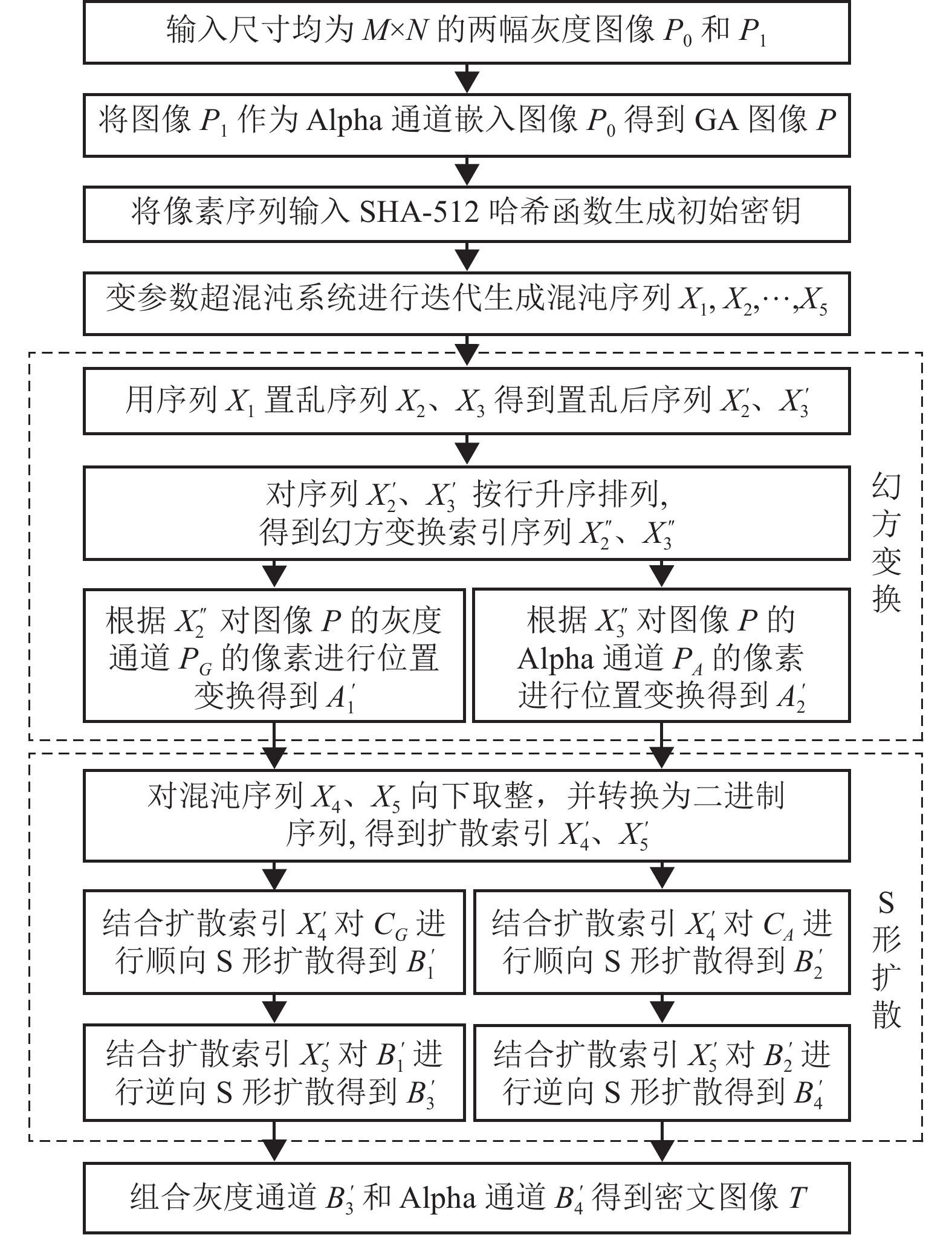
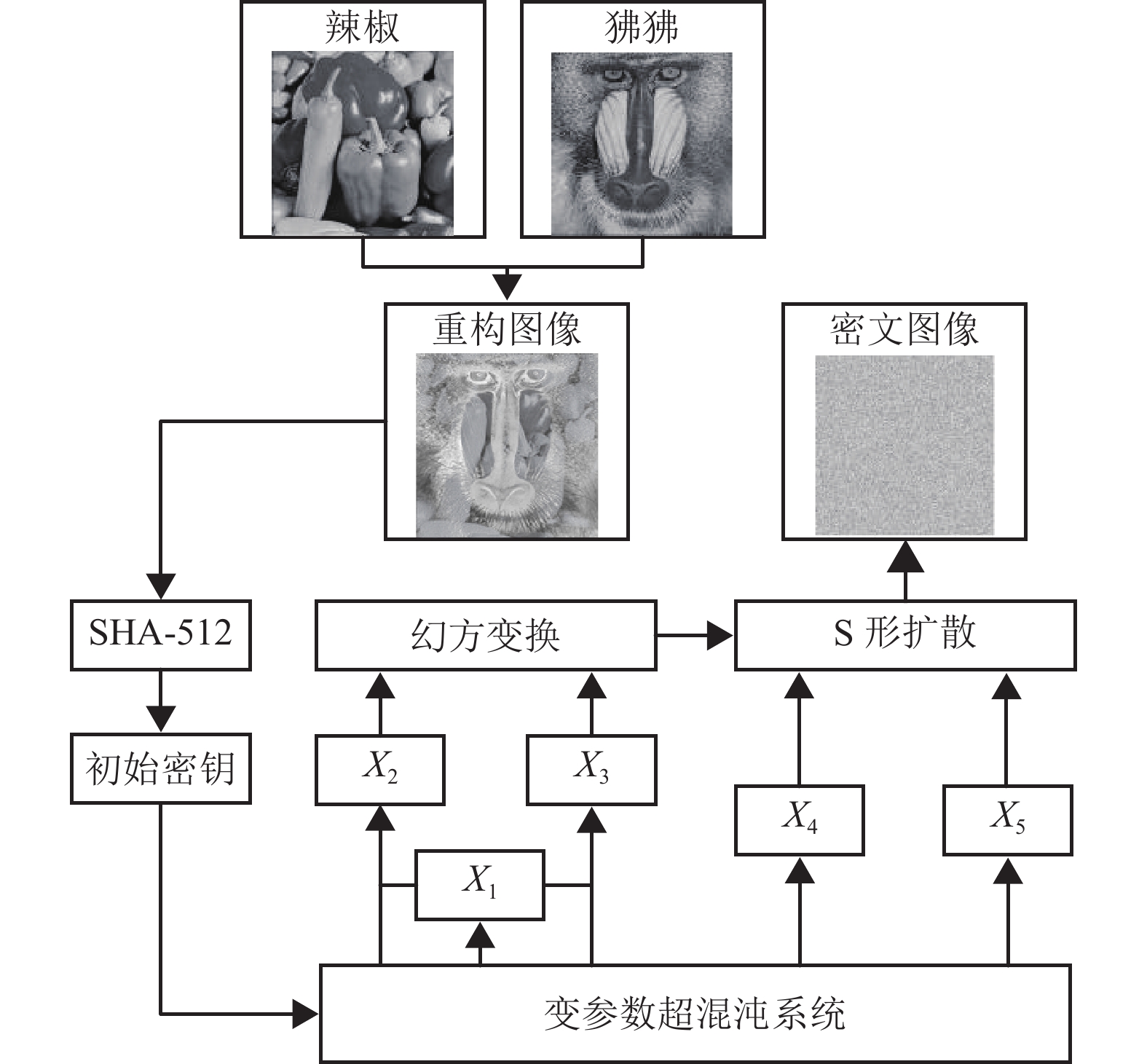
为了解决图像加密方法的上述问题,提供了一种基于变参数超混沌系统与S形扩散的多图像加密方法,如图1所示。首先借助Alpha通道的概念,将输入灰度图像(原始图像)进行重构,然后将其作为初始信息输入SHA-512算法生成初始密钥,再利用变参数超混沌系统迭代生成的5组混沌序列对明文图像进行幻方变换,实现像素位置的变换,最后基于S形扩散实现像素数值的变换,从而得到密文图像。具体技术方案包括以下3个步骤。
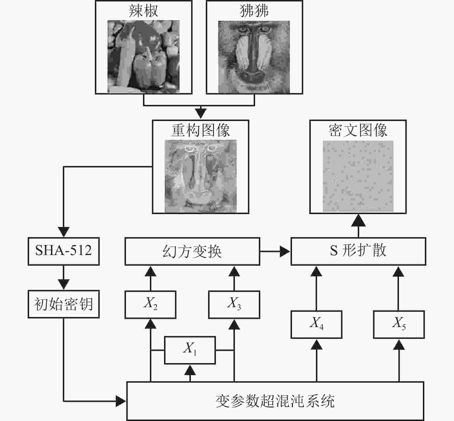
图 1 多图像加密方法的设计框架
1)首先对输入灰度图像对进行图像预处理,得到重构GA图像P,并将其像素序列作为初始信息输入SHA-512哈希函数生成初始密钥流;
2)再将初始密钥流作为初始值,输入变参数超混沌系统迭代生成混沌序列X1、X2、X3、X4与X5,并基于混沌序列X1、X2、X3计算得到索引序列;再根据索引序列对重构GA图像P采用幻方变换进行置乱,得到置乱后的密文图像C;
3)最后对密文图像C进行顺向S形扩散得到顺向扩散后矩阵,再对顺向扩散后矩阵进行逆向S形扩散,得到最终密文图像T。
-
根据Fan超混沌系统的定义[19],其数学模型如式(1)所示,其典型特征是:当a=30、b=10、c=15.7、d=5、e=2.5、f=4.45、g=38.5时,该混沌系统存在两个正的Lyapunov指数,即存在复杂的混沌行为。
$$ \left\{\begin{array}{l} \dot x_{1}=a\left(x_{2}-x_{1}\right)+x_{2} x_{3} x_{4} \\ \dot{x}_{2}=b\left(x_{1}+x_{2}\right)+x_{5}-x_{1} x_{3} x_{4} \\ \dot{x}_{3}=-c x_{2}-d x_{3}-e x_{4}+x_{1} x_{2} x_{4} \\ \dot x_{4}=-f x_{4}+x_{1} x_{2} x_{3} \\ \dot{x}_{5}=-g\left(x_{1}+x_{2}\right) \end{array}\right. $$ (1) 式中,x1、x2、x3、x4、x5为系统变量;a、b、c、d、e、f、g为系统参数;
$ \dot{x}_{1} $ 、$ \dot{x}_{2} $ 、$ \dot{x}_{3} $ 、$ \dot{x}_{4} $ 、$ \dot{x}_{5} $ 为每次迭代产生的新系统变量(Lyapunov指数)。为了增强混沌系统的复杂性和随机性,采用Logistic混沌映射作为扰动系统,对Fan超混沌系统的参数施加扰动来构造变参数混沌系统,以生成具有更高随机性的混沌序列,Logistic映射为非线性的迭代方程,如式(2)所示,其典型特征是:当满足3.57<µ<4时,Logistic映射工作于混沌状态,即为Logistic混沌映射。
$$ \dot{y}=\mu y (1-y) $$ (2) 式中,y为系统变量;μ为系统参数;
$ \dot{y} $ 为每次迭代产生的新系统变量。引入参数扰动项后的变参数超混沌系统的数学模型如式(3)所示,根据混沌系统的定义,无论初始值如何变化,系统变量都会回到一个固定的吸引域,由于式(1)、(2)均为混沌系统方程,因此Lyapunov指数的数值经过式(3)多次迭代后,只跟扰动强度λ有关,与y、xi (i=1,2,···,5)的初始值无关,y、xi的初始值可取实数范围内的任意值,最终稳定的Lyapunov指数的数值只依赖于扰动强度λ。
$$ \left\{\begin{array}{l} \dot{x}_{1}=(a+\lambda y) \left(x_{2}-x_{1}\right)+x_{2} x_{3} x_{4} \\ \dot{x}_{2}=(b+\lambda y) \left(x_{1}+x_{2}\right)+x_{5}-x_{1} x_{3} x_{4} \\ \dot{x}_{3}=-(c+\lambda y) x_{2}-d x_{3}-e x_{4}+x_{1} x_{2} x_{4} \\ \dot{x}_{4}=-(f+\lambda y) x_{4}+x_{1} x_{2} x_{3} \\ \dot{x}_{5}=-(g+\lambda y) \left(x_{1}+x_{2}\right) \end{array}\right. $$ (3) 式中,x1、x2、x3、x4、x5为系统变量;a、b、c、d、e、f、g为系统参数;
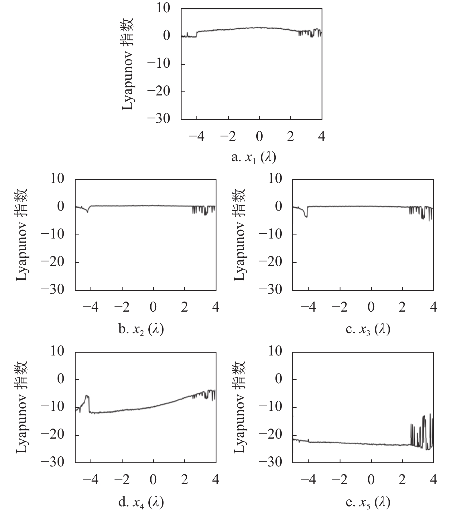
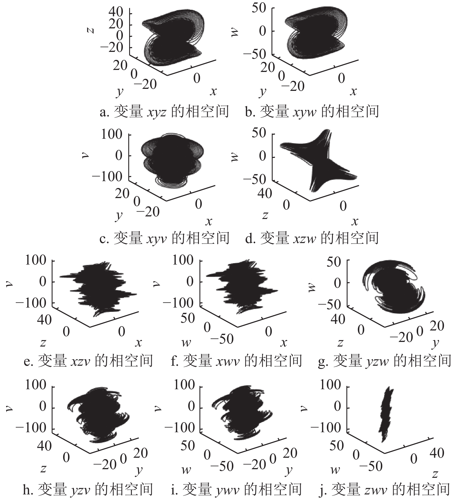
$ \dot{x}_{1} $ 、$ \dot{x}_{2} $ 、$ \dot{x}_{3} $ 、$ \dot{x}_{4} $ 、$ \dot{x}_{5} $ 为每次迭代产生的新系统变量;λ为扰动强度参数;y为Logistic混沌映射的系统参数。为了确定扰动强度参数λ的取值范围,确保变参数超混沌系统始终处于混沌状态,对变参数超混沌系统的Lyapunov指数和系统相图进行仿真分析,在系统参数a=30、b=10、c=15.7、d=5、e=2.5、f=4.45、g=38.5、μ=3.8时,取y=1、xi=0.1作为初始值,当变参数超混沌系统自身迭代300次后,Lyapunov指数的数值趋于稳定,将第301次迭代产生的y、xi以及系统参数代入式(3),得到了变参数超混沌系统(λ在−5~4之间变化)的Lyapunov指数变化曲线,如图2所示。当扰动强度参数λ在−4.0~2.35之间时,x1(λ)和x2(λ)始终大于零,即始终存在两个正的Lyapunov指数,使变参数超混沌系统保持混沌状态。图3给出了扰动强度参数λ为0时,变参数超混沌系统的系统相图,通过系统相图能够更直观地表现出变参数超混沌系统的动力学行为。
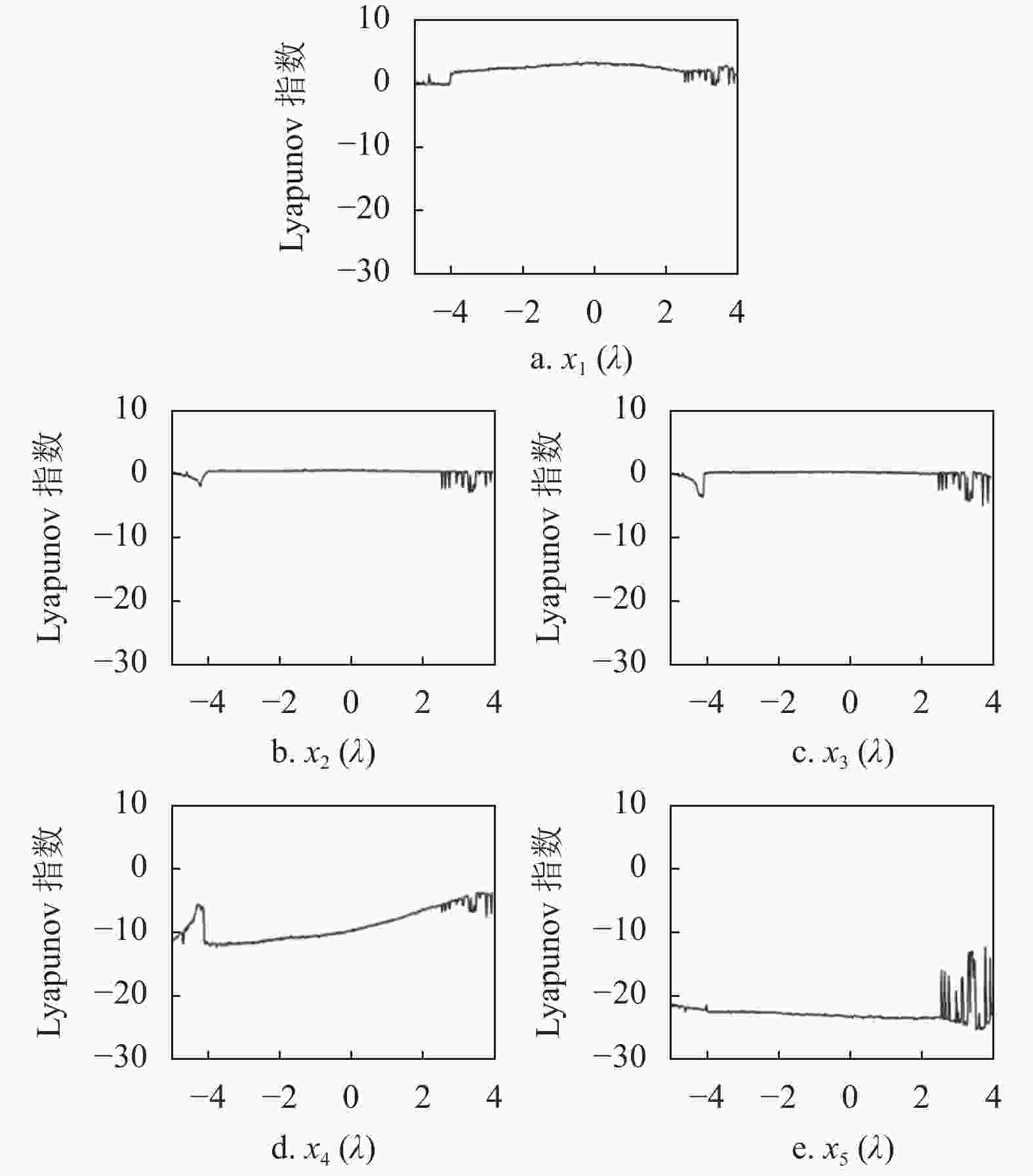
图 2 变参数超混沌系统的Lyapunov指数变化曲线
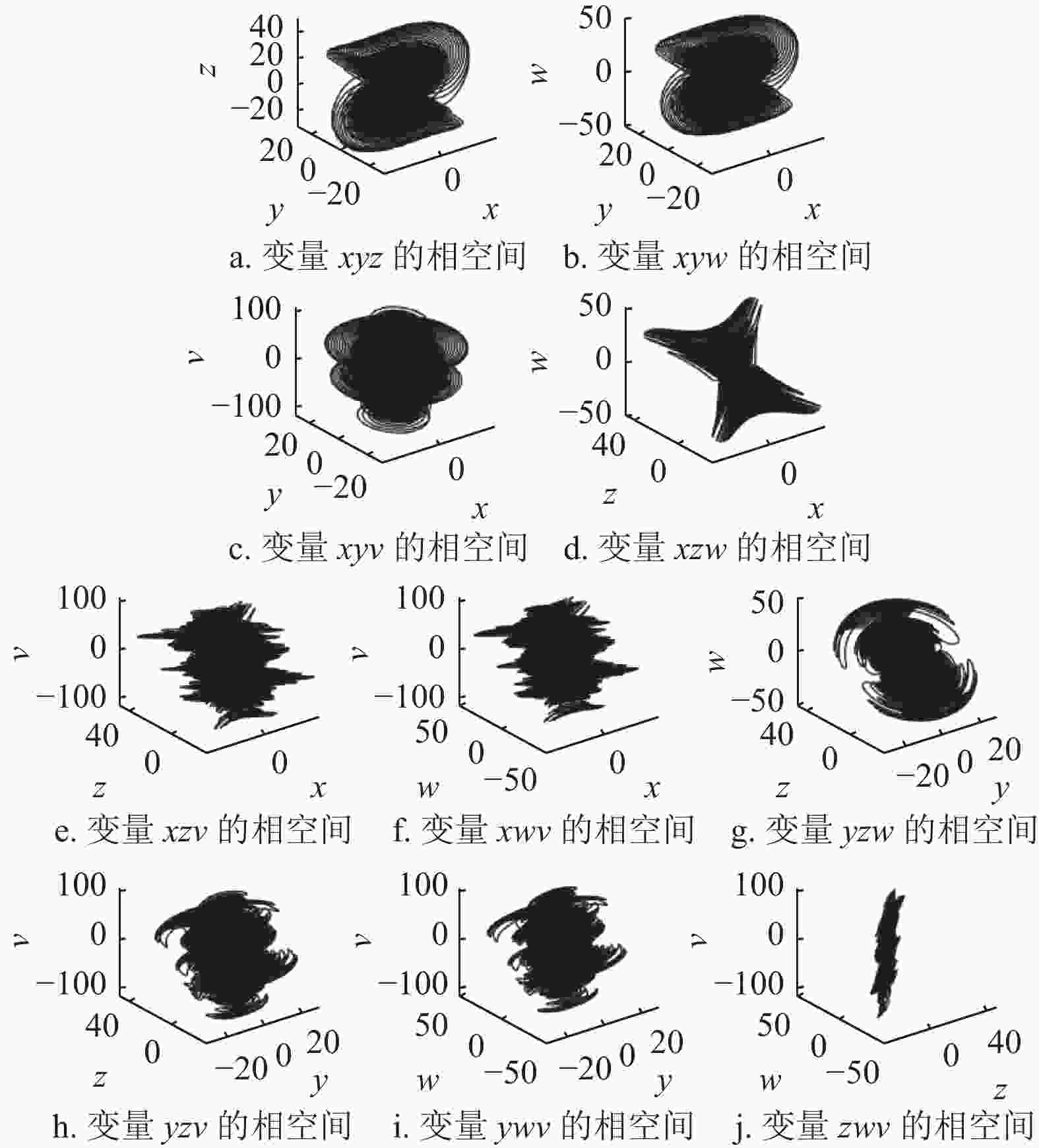
图 3 变参数超混沌系统的系统相图
-
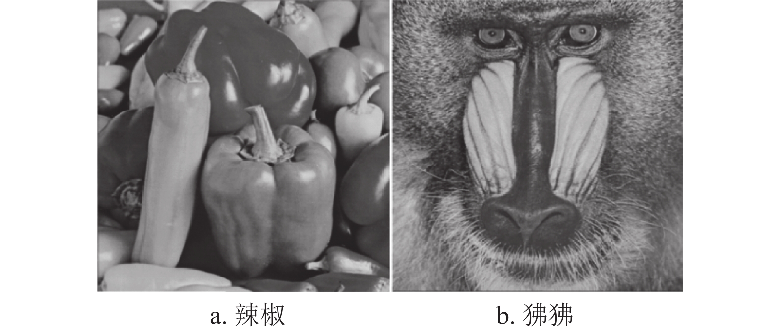
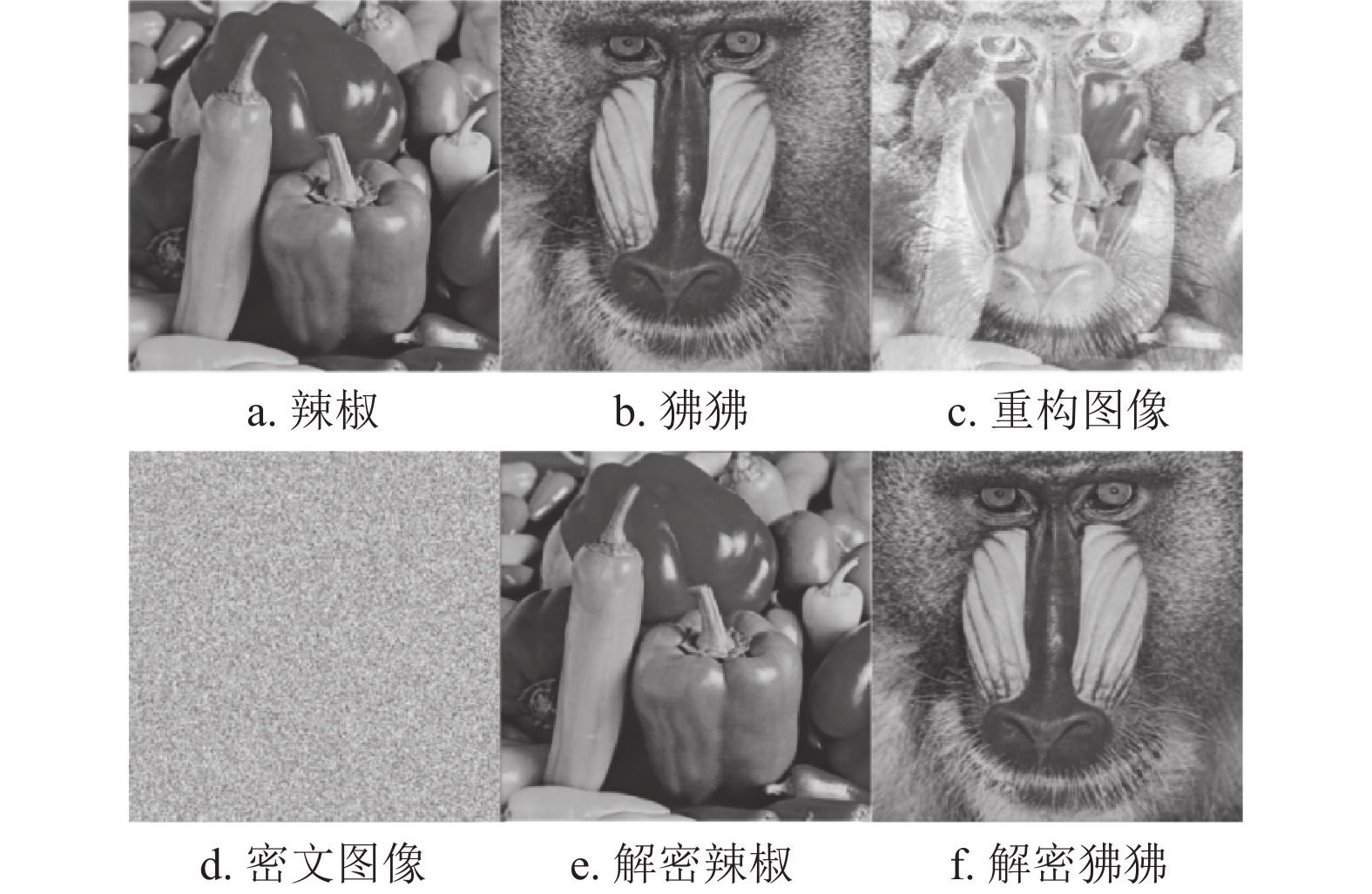
多图像加密方法的流程图如图4所示,包括图像预处理与密钥生成、置乱阶段和扩散阶段3个步骤。以下使用如图5所示的传统图像辣椒(灰度图像P0)与狒狒(灰度图像P1)为例进行说明,两张图像的像素大小均为512×512,记为M×N,M为图像像素长度、N为图像像素宽度。
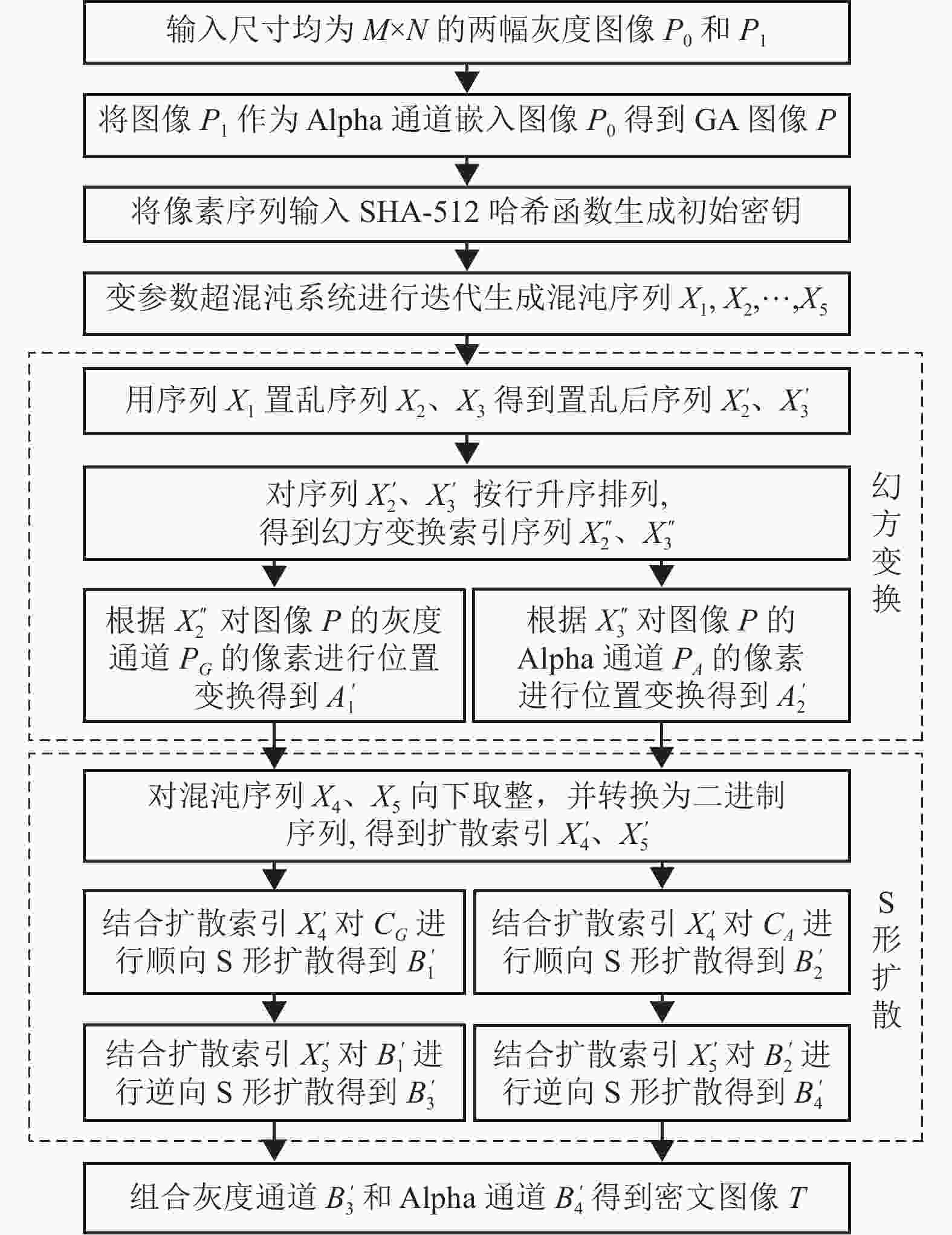
图 4 多图像加密方法的流程图
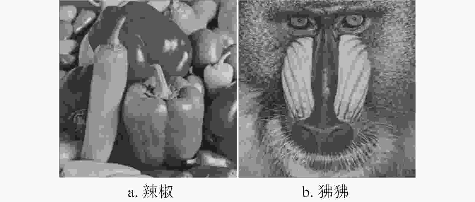
图 5 原始图像
-
1)引入Alpha通道的概念,将灰度图像P1作为Alpha通道嵌入至灰度图像P0,进而形成一幅具有不同透明度的Grayscale-Alpha(GA)图像P;
2)将图像P分解为灰度通道PG与Alpha通道PA两路数据矩阵(矩阵大小均为M×N),再将灰度通道PG与Alpha通道PA转换为一维矩阵,并拼接构成一维矩阵PC,将一维矩阵PC作为初始信息,输入SHA-512哈希函数,生成512 bit的二进制哈希值,具体运算为:
$$ P_{C}=\left[{ {\rm{reshape}} }\left(P_{G}, M \times N, 1\right) {, {\rm{reshape}} }\left(P_{A}, M \times N, 1\right)\right] $$ (4) 式中,reshape( )表示将指定矩阵变换为特定行列数的矩阵。
3)将二进制的哈希值以每8 bit为一位转化为十进制,进而得到64位十进制数据ci (i=1,2,···, 64);
4)对64位十进制数据进行异或运算得到加密方法所需要的初始密钥流,具体运算为:
$$ \left\{\begin{array}{l} \hat{x}_{1}=\dfrac{c_{1} \oplus c_{2} \oplus c_{3} \oplus \cdots \oplus c_{10}}{256} \\ \hat{x}_{2}=\dfrac{c_{11} \oplus c_{12} \oplus c_{13} \oplus \cdots \oplus c_{20}}{256} \\ \hat{x}_{3}=\dfrac{c_{21} \oplus c_{22} \oplus c_{23} \oplus \cdots \oplus c_{30}}{256} \\ \hat{x}_{4}=\dfrac{c_{31} \oplus c_{32} \oplus c_{32} \oplus \cdots \oplus c_{40}}{256} \\ \hat{x}_{5}=\dfrac{c_{41} \oplus c_{42} \oplus c_{43} \oplus \cdots \oplus c_{50}}{256} \\ \lambda=\text{mod} \left(\dfrac{c_{51} \oplus c_{52} \oplus c_{53} \oplus \cdots \oplus c_{64}}{256}, 6.35\right)-4 \end{array}\right. $$ (5) 式中,
$ \hat{x}_{1} $ 、$ \hat{x}_{2} $ 、$ \hat{x}_{3} $ 、$ \hat{x}_{4} $ 、$ \hat{x}_{5} $ 为初始密钥;$\oplus $ 表示异或操作;mod( )表示取余运算;需要说明的是:式(5)中λ的归一化过程能够保证其取值在−4.0~2.35之间,进而保证变参数混沌系统保持混沌状态。
-
1)根据初始密钥流,应用四阶龙格库塔算法对变参数超混沌系统进行迭代,为避免暂态效应的影响,舍弃前500组数据,从第501个数据进行截取,最终得到5组一维混沌序列X1、X2、X3、X4与X5,其中,每组混沌序列的长度均为M×N;
2)将混沌序列X1按行升序排列,得到置乱后矩阵I1与索引序列
$ {X}_{1}^{\prime} $ ,具体运算为:$$ \left[{\boldsymbol{I}}_{1}, X_{1}^{\prime}\right]={{\rm{sort}}}\left(X_{1}, 2, {{\rm{ascend}}}\right) $$ (6) 式中,sort( )表示排序函数;‘2’表示按行排序;
${\rm{ascend}}$ 表示升序排列;3)根据混沌索引序列
$ {X}_{1}^{\prime} $ ,对混沌序列X2、X3分别进行位置上的置乱,即根据混沌序列所对应索引序列相应位置的数值,将序列记录的数据移动到索引序列指定的位置,置乱示意图如图6所示;再对置乱后的混沌序列$ X_{2}^{\prime} $ 、$ X_{3}^{\prime} $ 按行升序排列,得到置乱后矩阵I2、I3与幻方变换所需的索引序列$ X_{2}^{\prime \prime} $ 、$X_{3}^{\prime \prime}$ ,具体运算为:$$ \left\{\begin{array}{l} {\left[{\boldsymbol{I}}_{2}, X_{2}^{\prime \prime}\right]={{\rm{sort}}}\left(X_{2}^{\prime}, 2, {{\rm{ascend}}}\right)} \\ {\left[{\boldsymbol{I}}_{3}, X_{3}^{\prime \prime}\right]={{\rm{sort}}}\left(X_{3}^{\prime}, 2, {{\rm{ascend}}}\right)} \end{array}\right. $$ (7) 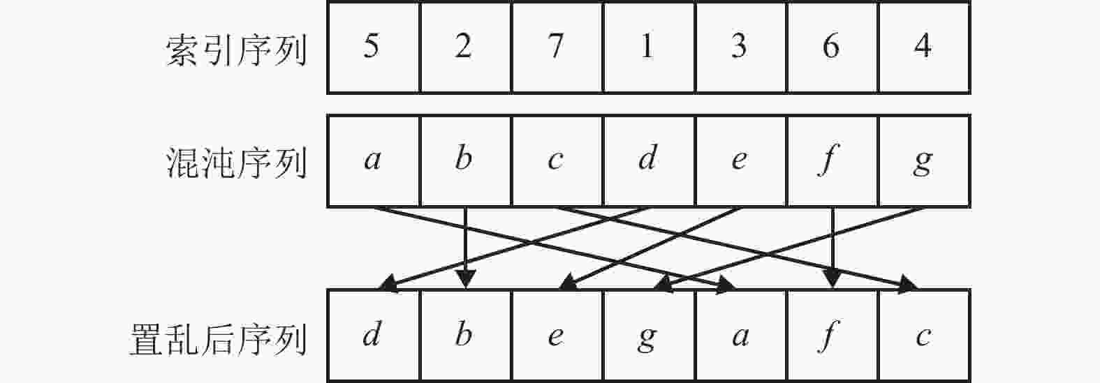
图 6 混沌序列置乱示意图
4)根据索引序列
$X_{2}^{\prime \prime}$ 、$X_{3}^{\prime \prime}$ ,分别对图像P的灰度通道PG与Alpha通道PA采用幻方变换进行置乱,对应得到置乱后的二维矩阵${\boldsymbol{A}}_{1}{}^{\prime}$ 、${\boldsymbol{A}}_{2}{}^{\prime}$ ,具体置乱过程如图7所示。以灰度通道PG为例,首先将灰度通道PG(二维矩阵)变换为一维序列$P_{{\rm{G}}}{}^{\prime}$ ,再根据索引序列$ X_{2}^{\prime \prime} $ 将序列$P_{\mathrm{G}}{}^{\prime}$ 中的像素移动到相应位置得到置乱后的一维序列A1,最后将置乱后的一维序列A1变换为置乱后的二维矩阵$A_{1}{}^{\prime}$ ,矩阵变换运算为:$$ \left\{\begin{array}{l} P_{G}^{\prime}={ {\rm{reshapd}} }\left(P_{G}, M \times N, 1\right) \\ A_{1}^{\prime}={{\rm{reshapd}}}\left(A_{1}, 1, M \times N\right) \end{array}\right. $$ (8) 式中,reshape( )表示将指定矩阵变换为特定行列数的矩阵。
5)将置乱后矩阵
$ {\boldsymbol{A}}_{1}^{\prime} $ 作为灰度通道,置乱后矩阵$ {\boldsymbol{A}}_{2}^{\prime} $ 作为Alpha通道,组合得到置乱后的密文图像C。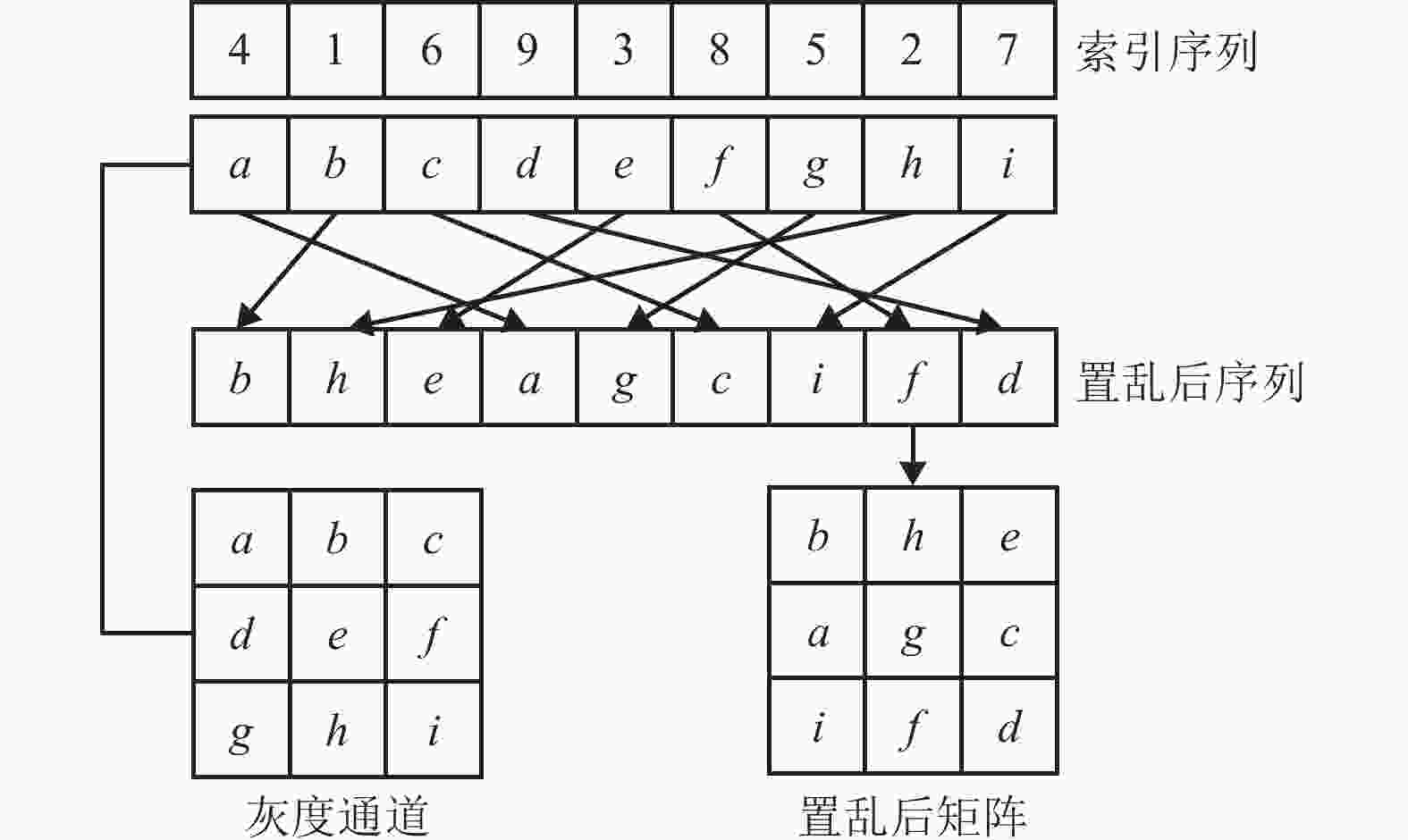
图 7 幻方变换示意图
-
1)将混沌序列X4与X5进行向下取整数运算,得到十进制整数的混沌序列,然后将十进制转换为二进制的一维序列
$ X_{4}^{\prime} $ 与$ X_{5}^{\prime} $ (长度均为M×8N):$$ \left\{\begin{array}{l} X_{4}^{\prime}={{\rm{dec}}} 2 {{\rm{bin}}}\left( {{\rm{floor}}}\left(X_{4}\right)\right) \\ X_{5}^{\prime}={{\rm{dec}}} 2 {{\rm{bin}}}\left( {{\rm{floor}}}\left(X_{5}\right)\right) \end{array}\right. $$ (9) 式中,dec2bin( )表示将十进制转换为二进制;floor( )为向下取整函数。
2)将密文图像C分解为灰度通道CG和Alpha通道CA两路数据矩阵(矩阵大小均为M×N),先对灰度通道CG和Alpha通道CA分别进行顺向S形扩散,再进行十进制到二进制的转换,得到二进制的一维矩阵
$C_{G}^{\prime}$ 与$c_{A}^{\prime}$ (长度均为M×8N);然后根据式(10)进行异或运算,得到二进制的一维矩阵B1与B2(长度均为M×8N),将二进制矩阵B1与B2转换为十进制矩阵,并将一维变换为二维,得到顺向扩散后矩阵$ B_{1}^{\prime} $ 与${B}_{2}^{\prime}$ (矩阵大小均为M×N):$$ \left\{\begin{array}{l} B_{1}(1)={ {\rm{floor}} }\left(\text{mod} \left(\displaystyle\sum_{j=1}^{M \times N} X_{4}(j), 2\right)\right) \oplus C_{G}^{\prime}(1) \oplus X_{4}^{\prime}(1) \\ B_{1}(i)=C_{G}^{\prime}(i-1) \oplus C_{G}^{\prime}(i) \oplus X_{4}^{\prime}(i)\;\;\;\; i=2,3, \cdots, M \times 8 N \\ B_{2}(1)={ {\rm{floor}} }\left(\text{mod} \left(\displaystyle\sum_{j=1}^{M \times N} X_{4}(j), 2\right)\right) \oplus C_{A}^{\prime}(1) \oplus X_{4}^{\prime}(1) \\ B_{2}(i)=C_{A}^{\prime}(i-1) \oplus C_{A}^{\prime}(i) \oplus X_{4}^{\prime}(i)\;\;\;\; i=2,3, \cdots, M \times 8 N \end{array}\right. $$ (10) $$ \left\{ {\begin{array}{*{20}{c}} {B_1^{'} = {\rm{reshape}}({\rm{bin}}2{\rm{dec}}({B_1}),1,M \times N)}\\ {B_2^{'} = {\rm{reshape}}({\rm{bin}}2{\rm{dec}}({B_2}),1,M \times N)} \end{array}} \right. $$ (11) 式中,mod( )表示取余运算;M、N为输入灰度图像的像素长度和像素宽度;bin2dec( )表示将二进制转换为十进制。
3)对矩阵
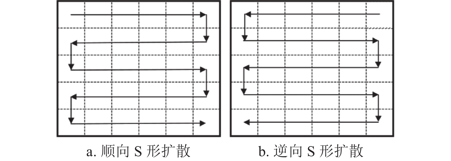
$ B_{1}^{\prime} $ 与$ B_{2}^{\prime} $ 分别进行逆向S形扩散,再进行十进制到二进制的转换,得到二进制的一维矩阵$ B_{1}^{\prime \prime} $ 与$ B_{2}^{\prime \prime} $ (长度均为M×8N);然后根据式(12)进行异或运算,得到二进制的一维矩阵B3与B4(长度均为M×8N),将二进制矩阵B3与B4转换为十进制矩阵,并将一维变换为二维,得到逆向扩散后矩阵$ B_{3}^{\prime} $ 与$ B_{4}^{\prime} $ (矩阵大小均为M×N),具体运算如式(13)所示;最后将二维矩阵$ B_{4}^{\prime} $ 作为Alpha通道嵌入二维矩阵$ B_{3}^{\prime} $ 中,得到最终密文图像T。$$ \left\{ {\begin{array}{*{20}{l}} {{B_3}\left( 1 \right) = {\rm{floor}}\left( {\text{mod} \left( {\displaystyle\sum\limits_{j = 1}^{M \times N} {{X_5}\left( j \right),2} } \right)} \right) \oplus B_1^{\prime \prime}\left( 1 \right) \oplus X_5^{'}\left( 1 \right)}\\ {{B_3}\left( i \right) = B_1^{\prime \prime}\left( {i - 1} \right) \oplus B_1^{\prime \prime}\left( i \right) \oplus X_5^{\prime}\left( i \right)\;\;\;\;i = 2,3, \cdots ,M \times 8N}\\ {{B_4}\left( 1 \right) = {\rm{floor}}\left( {\text{mod} \left( {\displaystyle\sum\limits_{j = 1}^{M \times N} {{X_5}\left( j \right),2} } \right)} \right) \oplus B_2^{\prime \prime}\left( 1 \right) \oplus X_5^{'}\left( 1 \right)}\\ {{B_4}\left( i \right) = B_2^{\prime \prime}\left( {i - 1} \right) \oplus B_2^{\prime \prime}\left( i \right) \oplus X_5^{\prime}\left( i \right)\;\;\;\;i = 2,3, \cdots ,M \times 8N} \end{array}} \right. $$ (12) $$ \left\{ {\begin{array}{*{20}{c}} {B_3^{\prime} = {\rm{reshape}}({\rm{bin}}2{\rm{dec}}({B_3}),1,M \times N)}\\ {B_4^{\prime} = {\rm{reshape}}({\rm{bin}}2{\rm{dec}}({B_4}),1,M \times N)} \end{array}} \right. $$ (13) 顺向S形扩散的定义如图8a所示,具体运算为:
$$ \left\{ {\begin{array}{*{20}{c}} {Q{'} = {S_{{\rm{forward}}}}\left( {\boldsymbol{Q}} \right)}\\ {{\boldsymbol{Q}} = \left[ {\begin{array}{*{20}{c}} {{q_{1,1}}}&{{q_{1,2}}}& \cdots &{{q_{1,N}}}\\ {{q_{2,1}}}&{{q_{2,2}}}&\cdots &{{q_{2,N}}}\\ \vdots & \vdots &{}& \vdots \\ {{q_{M,1}}}&{{q_{M,2}}}& \cdots &{{q_{M,N}}} \end{array}} \right]}\\ Q{'} = \left[ {q_{1,1}},{q_{1,2}}, \cdots ,{q_{1,N}},{q_{2,N}},{q_{2,N-1}}, \cdots ,{q_{2,1}},{q_{3,1}},\right. \\ \left.{q_{3,2}}, \cdots ,{q_{3,N}},{q_{4,N}}, \cdots \right] \end{array}} \right. $$ (14) 式中,Sforward( )表示顺向S形扩散运算;Q为原始矩阵;
$ Q^{\prime} $ 为顺向S形扩散结果。逆向S形扩散的定义如图8b所示,具体运算为:
$$ \left\{ {\begin{array}{*{20}{c}} {Q^{\prime \prime }= {S_{{\rm{reverse}}}}\left( {\boldsymbol{Q}} \right)}\\ {{\boldsymbol{Q}} = \left[ {\begin{array}{*{20}{c}} {{q_{1,1}}}&{{q_{1,2}}}& \cdots &{{q_{1,N}}}\\ {{q_{2,1}}}&{{q_{2,2}}}& \cdots &{{q_{2,N}}}\\ \vdots & \vdots &{}& \vdots \\ {{q_{M,1}}}&{{q_{M,2}}}& \cdots &{{q_{M,N}}} \end{array}} \right]}\\ Q^{\prime \prime }= \left[ {q_{1,N}},{q_{1,N - 1}}, \cdots ,{q_{1,1}},{q_{2,1}},{q_{2,2}}, \cdots ,{q_{2,N}},{q_{3,N}},\right. \\ \left.{q_{3,N - 1}}, \cdots ,{q_{3,1}},{q_{4,1}}, \cdots \right] \end{array}} \right. $$ (15) 式中,Sreverse( )表示逆向S形扩散运算;Q为原始矩阵;
$ Q^{\prime \prime} $ 为逆向S形扩散结果。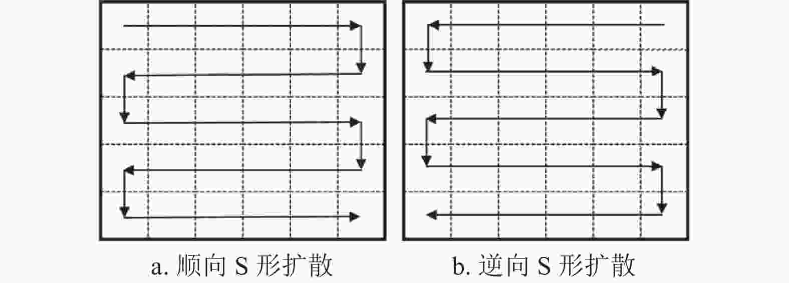
图 8 顺向和逆向S形扩散示意图
-
图像解密方法使用与加密方法相同的密钥,具体包括以下3个步骤。
1)将密文图像分解为两通道十进制数据矩阵,即灰度通道J与Alpha通道K(矩阵大小均为M×N),对J与K分别进行顺向S形扩散的逆操作,再进行十进制到二进制的转换,得到二进制的一维矩阵
${{\boldsymbol{J}}^{\prime}}$ 与$ {\boldsymbol{K}}^{\prime} $ (长度均为M×8N);根据式(16)进行异或运算,得到二进制的一维矩阵J1和K1(长度均为M×8N),将二进制矩阵J1和K1转换为十进制矩阵,并将其变换为二维矩阵$ {\boldsymbol{J}}_{1}^{\prime} $ 与$ {{\boldsymbol{K}}}_{1}^{\prime} $ (矩阵大小均为M×N),具体运算如式(17)所示:$$ \left\{ {\begin{array}{*{20}{c}} {{J_1}\left( 1 \right) = {\rm{floor}}\left( {\text{mod} \left( {\displaystyle\sum\limits_{j = 1}^{M \times N} {{X_4}\left( j \right),2} } \right)} \right) \oplus J{'}\left( 1 \right) \oplus X_4{'}\left( 1 \right)}\\ {{J_1}\left( i \right) = J{'}\left( {i - 1} \right) \oplus J'\left( i \right) \oplus X_4{'}\left( i \right)\;\;\;\;i = 2,3, \cdots ,M \times 8N}\\ {{K_1}\left( 1 \right) = {\rm{floor}}\left( {\text{mod} \left( {\displaystyle\sum\limits_{j = 1}^{M \times N} {{X_4}\left( j \right),2} } \right)} \right) \oplus K{'}\left( 1 \right) \oplus X_4{'}\left( 1 \right)}\\ {{K_1}\left( i \right) = K{'}\left( {i - 1} \right) \oplus K{'}\left( i \right) \oplus X_4{'}\left( i \right)\;\;\;\;i = 2,3, \cdots ,M \times 8N} \end{array}} \right. $$ (16) $$ \left\{\begin{array}{l} {\boldsymbol{J}}_{1}^{\prime}={ {\rm{reshape}} }\left({ {\rm{bin}}2{\rm{dec}} }\left(J_{1}\right), 1, M \times N\right) \\ {\boldsymbol{K}}_{1}^{\prime}={ {\rm{reshape}} }\left({ {\rm{bin}}2{\rm{dec}} }\left(K_{1}\right), 1, M \times N\right) \end{array}\right. $$ (17) 2)对矩阵
$ {\boldsymbol{J}}_{1}^{\prime} $ 与${{\boldsymbol{K}}}_{1}^{\prime} $ 分别进行逆向S形扩散的逆操作,再进行十进制到二进制的转换,得到二进制的一维矩阵$ {\boldsymbol{J}}_{1}^{\prime \prime} $ 与$ {\boldsymbol{K}}_{1}^{\prime \prime} $ (长度均为M×8N);根据式(18)进行异或运算,得到二进制的一维矩阵J2和K2(长度均为M×8N),将二进制矩阵J2和K2转换为十进制矩阵,并将其变换为二维矩阵$ {\boldsymbol{J}}_{2}^{\prime} $ 与$ {\boldsymbol{K}}_{2}^{\prime} $ (矩阵大小均为M×N):$$ \left\{\begin{array}{l} J_{2}(1)={ {\rm{floor}} }\left(\text{mod} \left(\displaystyle\sum_{j=1}^{M \times N} X_{5}(j), 2\right)\right) \oplus J_{1}^{\prime \prime}(1) \oplus X_{5}^{\prime}(1) \\ J_{2}(i)=J_{1}^{\prime \prime}(i-1) \oplus J_{1}^{\prime \prime}(i) \oplus X_{5}^{\prime}(i)\;\;\;\; i=2,3, \cdots, M \times 8 N \\ K_{2}(1)={ {\rm{floor}} }\left(\text{mod} \left(\displaystyle\sum_{i=1}^{M \times N} X_{5}(j), 2\right)\right) \oplus K_{1}^{\prime \prime}(1) \oplus X_{s}^{\prime}(1) \\ K_{2}(i)=K_{1}^{\prime \prime}(i-1) \oplus K_{1}^{\prime \prime}(i) \oplus X_{5}^{\prime}(i)\;\;\;\; i=2,3, \cdots, M \times 8 N \end{array}\right. $$ (18) $$ \left\{ {\begin{array}{*{20}{c}} {{\boldsymbol{J}}_2^{\prime} = {\rm{reshape}}({\rm{bin}}2{\rm{dec}}({{\boldsymbol{J}}_2}),1,M \times N)}\\ {{\boldsymbol{K}}_2^{\prime} = {\rm{reshape}}({\rm{bin}}2{\rm{dec}}({{\boldsymbol{J}}_2}),1,M \times N)} \end{array}} \right. $$ (19) 3)对
$ {\boldsymbol{J}}_{2}^{\prime} $ 与$ {\boldsymbol{K}}_{2}^{\prime} $ 进行逆幻方运算,得到十进制的二维矩阵J3与K3(矩阵大小均为M×N),矩阵J3对应灰度通道,即为原始图像P0,矩阵K3对应Alpha通道,即为原始图像P1。 -
通过上述多图像加解密方法,对如图5所示的传统图像辣椒与狒狒进行加解密实验,得到的仿真图如图9所示。由图可见,密文图像是完全无序的,无法分辨出原始图像的任何有效信息。
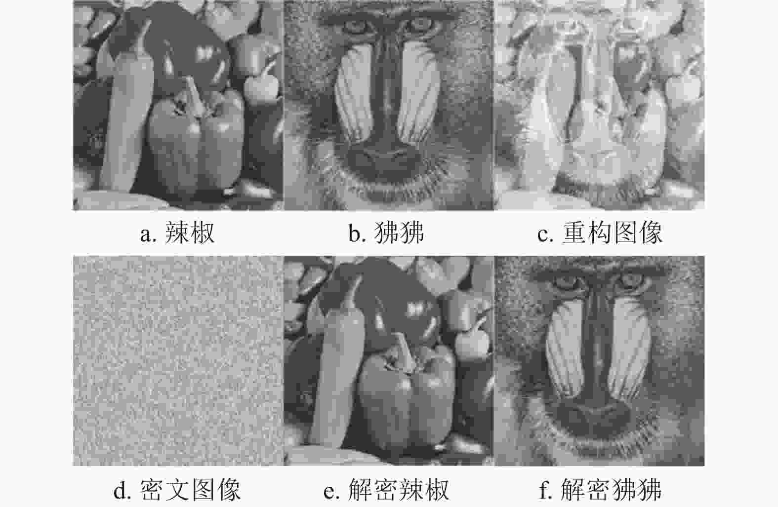
图 9 原始图像加解密实验的结果展示图
-
为了验证多图像加密方法的安全性能,图10给出了加解密前后的直方图;由图可见,图像辣椒与图像狒狒的密文图像直方图均近似均匀分布,攻击者很难从中获取有效信息。
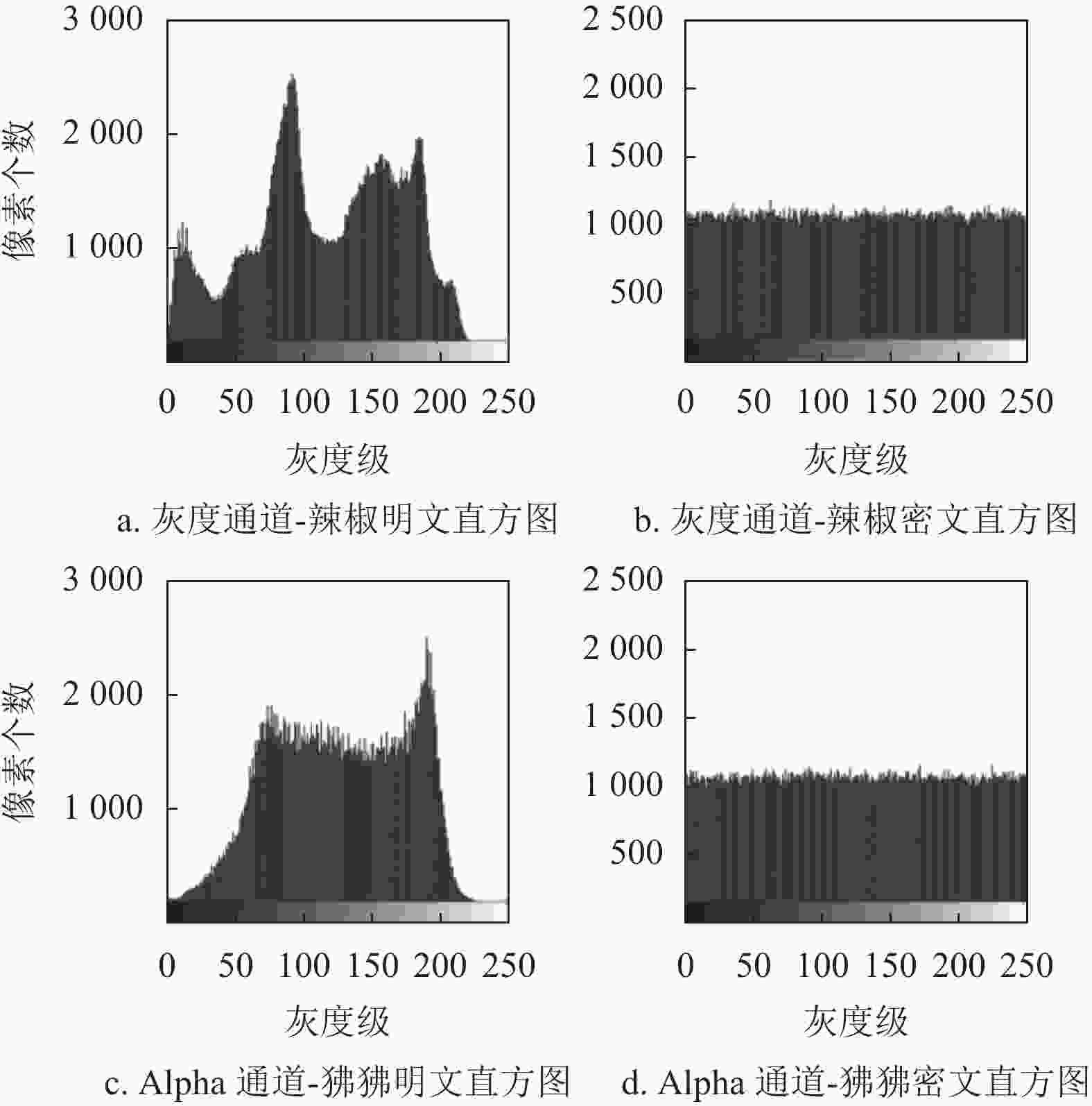
图 10 灰度通道和Alpha通道的明文和密文直方图
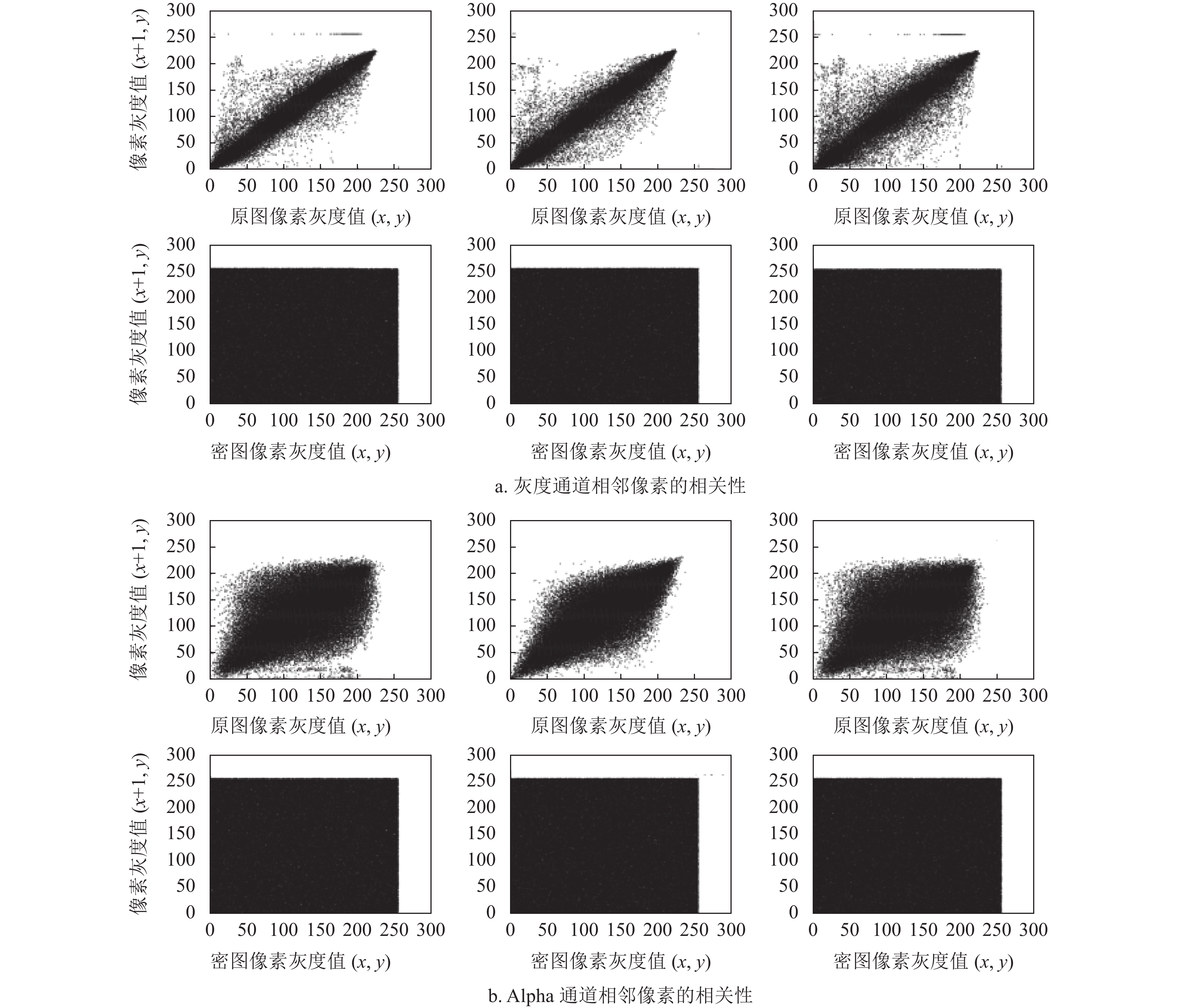
此外,为了更加直观地说明多图像加密方法打破相邻像素相关性的能力,图11给出了加密前后灰度通道与Alpha通道的像素相关性分布图。由图可见,加密后的相关性分布遍布整个区域,有效地破坏了明文图像的像素相关性分布。
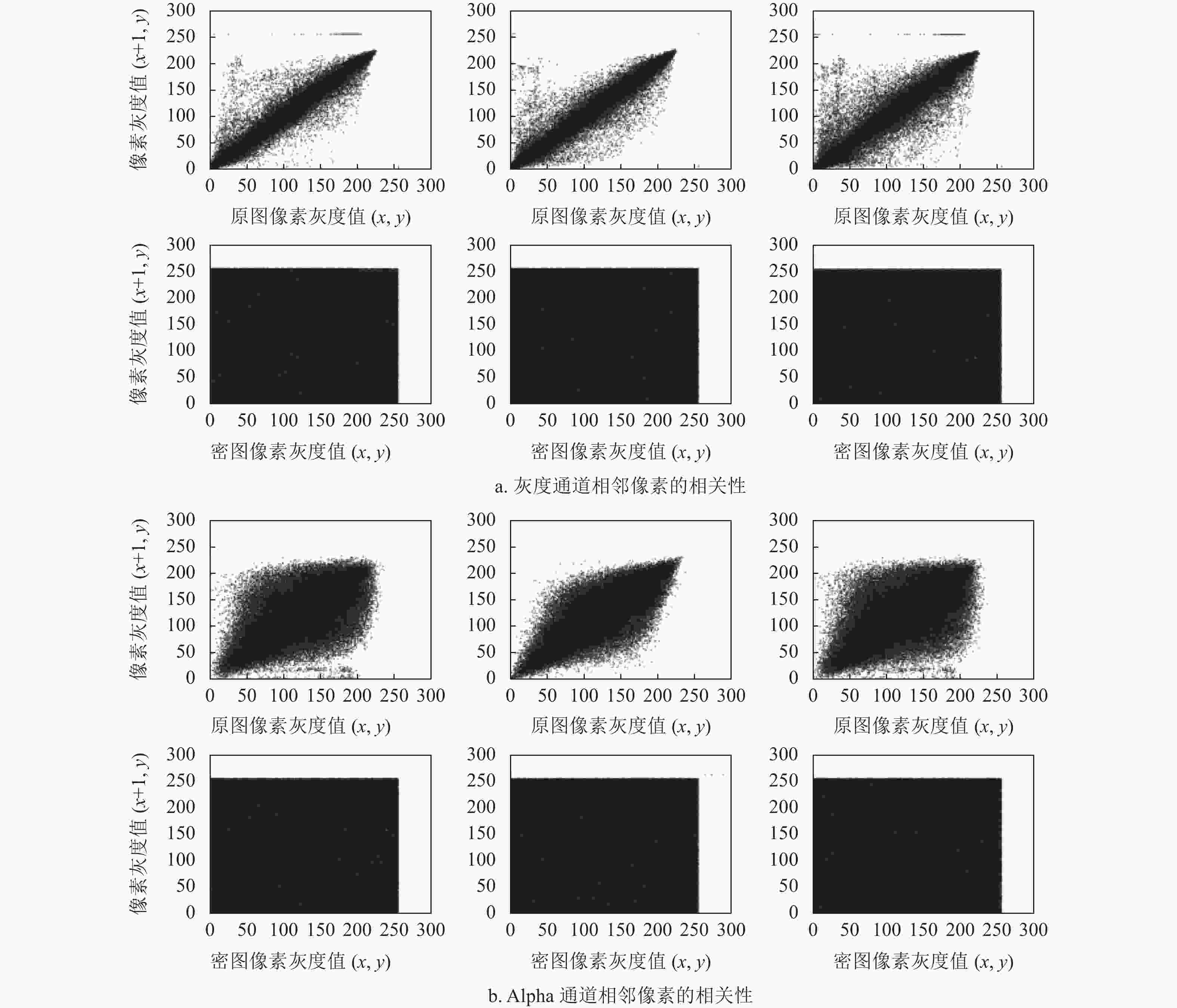
图 11 灰度通道和Alpha通道的明文和密文相邻像素相关性对比图
信息熵用于表征一个数字图像像素的分布情况,信息熵越接近理想值8,像素分布越随机。为验证加密算法扰乱明文图像像素分布的能力,对辣椒和狒狒加密前后图像进行信息熵分析。表1给出了经加密算法加密后,明文图像与密文图像的信息熵。可以看出,密文图像的信息熵接近理想值8,这证明设计的加密算法可以更加有效地打乱明文像素分布。
表 1 信息熵分析表
图像 明文信息熵 密文信息熵 辣椒 6.7961 7.9992 狒狒 6.5044 7.9993 加密算法的抗差分攻击能力主要体现在对同一明文图像任一像素点施加微小改变,密文图像随之产生相应变化的能力。本文将明文图像某一像素点的像素值减1,然后通过计算NPCR和UACI,对抗差分攻击能力进行评估,结果如表2所示。可以看出,加密算法的NPCR和UACI接近理想值99.6094%和33.4635%,说明设计的加密算法对明文的微小变化具有更高的敏感性,可以更加有效地抵御差分攻击。
表 2 抗差分攻击能力分析表
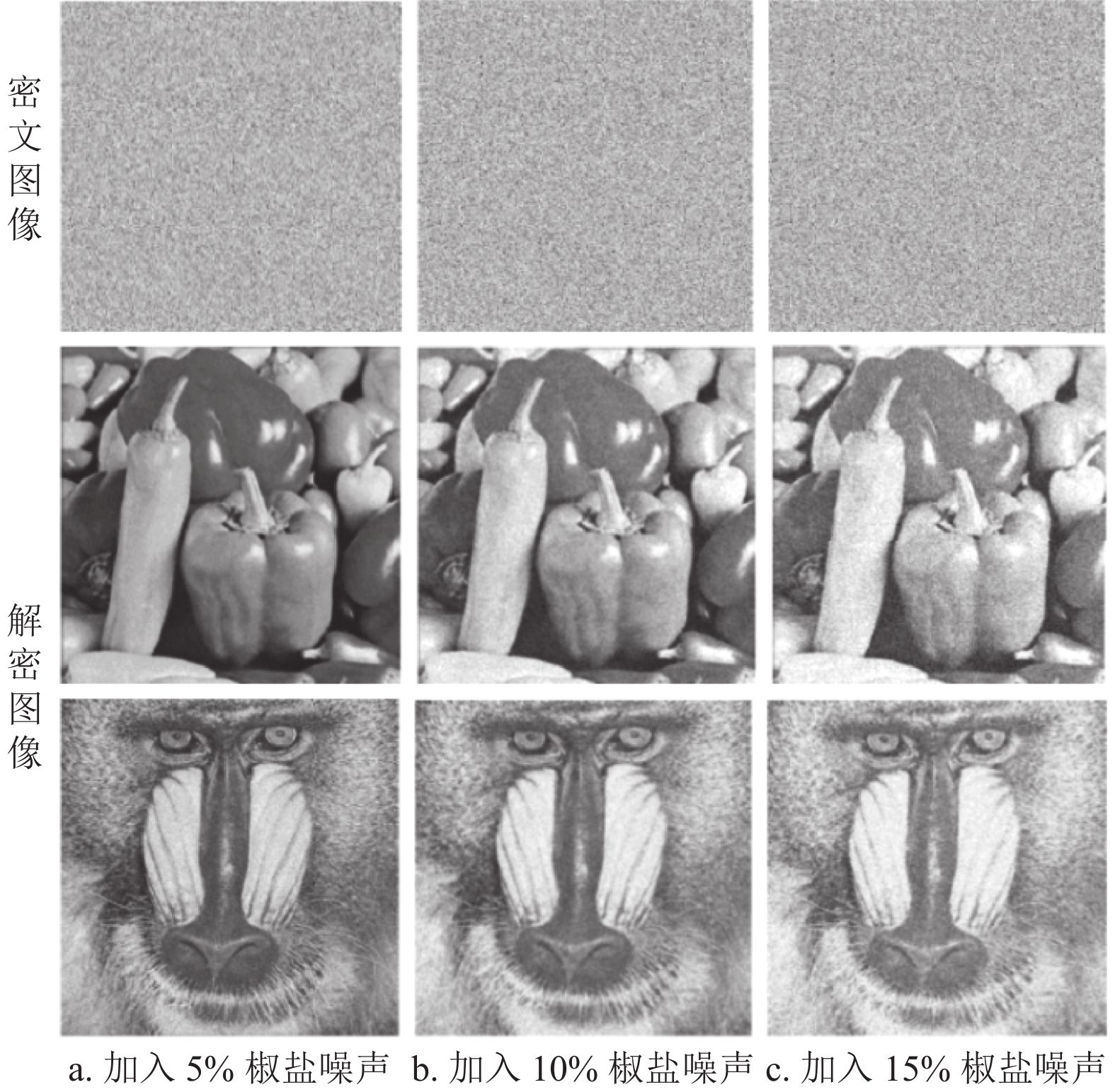
% 图像 NPCR UACI 辣椒 99.60 33.49 狒狒 99.63 33.48 当图像进行网络传输时,可能会引入各种噪声干扰,导致密文图像某些像素点的像素值发生改变,进而影响到原始图像有效信息的恢复。本文对辣椒和狒狒加密后的密文图像分别加入5%、10%和20%的椒盐噪声,以此验证加密算法的抗噪声能力。图12为辣椒和狒狒引入椒盐噪声后的密文图像以及运用解密算法解密后的图像。可以看出,引入不同程度的椒盐噪声后,解密图像虽然受到一定程度的损坏,但是依旧可以分辨出大部分有效信息,因此所提加密算法具有良好的抗噪声能力。
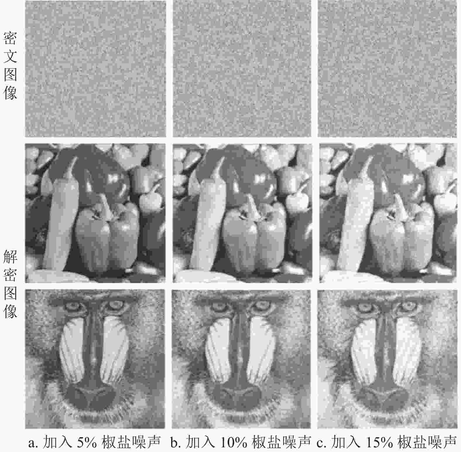
图 12 算法性能对比:抗噪声分析
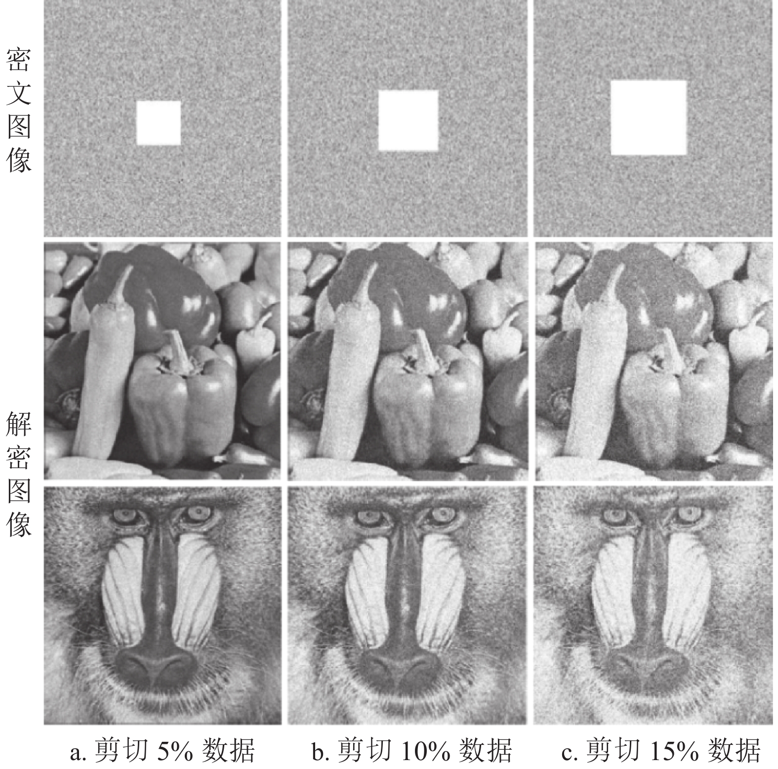
为验证加密算法的抗剪切能力,本文将辣椒和狒狒加密后的密文图像,在不同位置剪切不同像素大小的信息,然后再对其进行解密,剪切后的密文图像以及相应的解密图像如图13所示。从图中可以看出,密文图像受到人为剪切后,加密算法仍然可以恢复出原始图像的主要信息,具备良好的抗剪切能力。

图 13 算法性能对比:抗剪切分析
-
基于变参数超混沌系统的多图像加密方法,主要由4个部分构成:变参数超混沌系统构建、图像预处理与密钥生成、幻方变换置乱和S形扩散。首先借助Alpha通道的概念,将输入灰度图像对进行重构,然后将重构图像作为初始信息输入SHA-512算法生成初始密钥,再将其输入变参数超混沌系统迭代生成5组混沌序列,进而对重构图像进行幻方变换,实现像素位置的变换,最后基于S形扩散实现像素数值的变化,从而得到密文图像。
与传统图像加密方法相比,基于变参数超混沌系统的多图像加密方法,具有如下优点:
1)将混沌系统的参数作为加密过程中的控制变量之一,运用另一个混沌系统的状态变量对其施加一定的扰动,以构造变参数超混沌系统,同时确保该混沌系统依旧处于混沌状态,生成具有更高复杂度和随机性的伪随机序列,有效地改善了传统混沌系统的低随机性、低复杂度以及混沌系统退化等缺陷;
2)采用幻方变换的置乱方法,最大程度地对图像像素进行位置上的置乱,并创造性地提出S形扩散方法,提高了密文图像的无序性,打破了像素相关性分布,具有更优越的加密性能表现,难以被暴力破译;
3)采用SHA-512算法,结合明文图像生成初始密钥,保证一幅图像仅仅对应一种密钥流,有效地提高了加密算法抵抗明文攻击的能力;
4)本文设计的加密算法可以有效地打乱明文像素分布、有效地抵御差分攻击,具有良好的抗噪声能力和具备良好的抗剪切能力。
Multi-Image Encryption Method Based on Hyperchaotic System with Variable Parameters
-
摘要: 针对数字图像计算、存储和传输过程中的数据窃取、隐私泄漏等问题,提出了一种基于变参数超混沌系统的多图像加密方法。首先,用一个混沌系统的状态变量对另一个混沌系统的状态参数施加扰动,构造了一个变参数超混沌系统;其次,将输入灰度图像对进行重构,并将其输入SHA-512算法生成初始密钥;然后,将初始密钥输入变参数超混沌系统,迭代生成5组混沌序列,进而对重构图像进行幻方变换,实现像素位置的变换;最后,对幻方变换得到的图像进行S形扩散,实现像素数值的变化,得到了近似均匀分布的密文图像。结果表明,该算法改善了传统图像加密方法的低随机性、低复杂度等缺陷,同时,提高了密文图像的无序性及抵抗常规攻击的能力。Abstract: Aiming at the problems of data theft and privacy leakage in the process of digital image calculation, storage and transmission, a multi-image encryption method based on hyperchaotic system with variable parameters is proposed. Firstly, the state variables of one chaotic system are used to perturb the state parameters of the other chaotic system, and a hyperchaotic system with variable parameters is constructed. Secondly, the input gray image pair is reconstructed and input into SHA-512 algorithm to generate the initial key. Then, the initial key is input into the hyperchaotic system with variable parameters to generate five groups of chaotic sequences iteratively, and then the reconstructed image is transformed into a magic square to achieve the transformation of pixel positions. Finally, the S-shaped diffusion is performed on the image obtained by the magic square transformation to realize the change of the pixel value, and an approximately uniformly distributed ciphertext image is obtained. The results show that the algorithm improves the low randomness and low complexity of the traditional image encryption method, and at the same time, and improves the disorder of the ciphertext image and the ability of the encryption method to resist conventional attacks.
-
Key words:
- hyperchaotic system /
- image encryption /
- magic square transformation /
- S-shaped diffusion
-
[1] WANG X, ZHAO M. An image encryption algorithm based on hyper-chaotic system and DNA coding[J]. Optics and Laser Technology, 2021, 143: 107316. doi: 10.1016/j.optlastec.2021.107316 [2] XUE Q Y, LUO Y L, LIU J X, et al. A color image encryption method based on memristive hyperchaotic system and DNA encryption[J]. International Journal of Modern Physics B, 2020, 34: 2050014. doi: 10.1142/S0217979220500149 [3] HOSNY K M, KAMAL S T, DARWISH M M, et al. New image encryption algorithm using hyperchaotic system and fibonacci Q-matrix[J]. Electronics, 2021, 10: 1066. doi: 10.3390/electronics10091066 [4] ZHOU S, WANG X Y, ZHANG Y Q. Novel image encryption scheme based on chaotic signals with finite precision error[J]. Information Sciences, 2022, 22: 01395. [5] GAO X Y, YU J W, BANERJEE S, et al. A new image encryption scheme based on fractional-order hyperchaotic system and multiple image fusion[J]. Scientific Reports, 2021, 11: 15737. doi: 10.1038/s41598-021-94748-7 [6] SHEELA S J, SANJAY A, SURESH K V, et al. Image encryption based on 5D hyperchaotic system using hybrid random matrix transform[J]. Multidimensional Systems and Signal Processing, 2022, 33: 579-595. doi: 10.1007/s11045-021-00814-8 [7] HUI Y Y, LIU H, FANG P F. A DNA image encryption based on a new hyperchaotic system[J]. Multimedia Tools and Applications, 2021, 82: 21983-22007. [8] WANG Y Z, YANG F F. A fractional-order CNN hyperchaotic system for image encryption algorithm[J]. Physica Scripta, 2021, 96: 035209. doi: 10.1088/1402-4896/abd50f [9] QI G Y, VAN WYK M A, VAN WYK B J, et al. On a new hyperchaotic system[J]. Physics Letters A, 2008, 372: 124-136. doi: 10.1016/j.physleta.2007.10.082 [10] FAN C L, DING Q. A universal method for constructing non-degenerate hyperchaotic systems with any desired number of positive Lyapunov exponents[J]. Chaos, Solitons and Fractals, 2022, 161: 112323. doi: 10.1016/j.chaos.2022.112323 [11] WU L L, ZHANG J W, DENG W T, et al. Arnold transformation algorithm and anti-arnold transformation algorithm[C]//1st International Conference on Information Science and Engineering. [S.l.]: IEEE, 2009: 1164-1167. [12] WANG X Y, SUN H H, GAO H. An image encryption algorithm based on improved baker transformation and chaotic S-box[J]. Chinese Physics B, 2021, 30: 060507. doi: 10.1088/1674-1056/abdea3 [13] WANG J, LIU L F. A novel chaos-based image encryption using magic square scrambling and octree diffusing[J]. Mathematics, 2022, 10: 457. doi: 10.3390/math10030457 [14] HERBADJI D, DEROUICHE N, BELMEGUENAI A, et al. A tweakable image encryption algorithm using an improved logistic chaotic map[J]. Traitement du Signal, 2019, 36: 407-417. doi: 10.18280/ts.360505 [15] LIU L D, JIANG D H, WANG X Y, et al. 2D logistic-adjusted-chebyshev map for visual color image encryption[J]. Journal of Information Security and Applications, 2021, 60: 102854. doi: 10.1016/j.jisa.2021.102854 [16] ZOU C Y, ZHANG Q, WEI X P, et al. Image encryption based on improved lorenz system[J]. IEEE Access, 2020, 60: 75728-75740. [17] LIN R G, LI S. An image encryption scheme based on lorenz hyperchaotic system and RSA algorithm[J]. Security and Communication Networks, 2021, 5: 1-18. [18] CHEN G R, MAO Y B, CHUI C K. A symmetric image encryption scheme based on 3D chaotic cat maps[J]. Chaos, Solitons and Fractals, 2004, 21: 749-761. doi: 10.1016/j.chaos.2003.12.022 [19] FAN B, TANG L R. A new five-dimensional hyperchaotic system and its application in DS-CDMA[C]//9th International Conference on Fuzzy Systems and Knowledge Discovery. [S.l.]: IEEE, 2012: 2069-2073. -

 点击查看大图
图(13) / 表(2)
计量
- 文章访问数: 4711
- HTML全文浏览量: 1245
- PDF下载量: 33
- 被引次数: 0