The following notations are used throughout the paper. N denotes the set of all natural numbers (including zero), R denotes the set of all real numbers, and Φ denotes the empty set. For l, l'∈R, max(l, l') denotes the larger one between l and l'. For a set π, |π| denotes the number of elements of π, π^∞ denotes both finite and infinite sequences over π. A closed interval is denoted with square brackets. For example [0, 1] means greater than or equal to 0 and less than or equal to 1. The infimum (or supremum) of a subset S of real numbers is denoted by inf(S) (or sup(S)) and is defined to be the largest (or least) real number which is smaller (or greater) than or equal to all numbers in S.

Definition 1 A metric on a set π is a function (called the distance function) d:π×π→[0, +∞] such that ∀x, y, z∈π,

1) d(x, y)=0 iff (if and only if) x=y (identity of indiscernibles);

2) d(x, y)=d(y, x) (symmetry);

3) d(x, z)≤d(x, y)+d(y, z) (triangular inequality).

Definition 2 A pseudo-metric on a set π is a function d:π×π→[0, +∞] such that:

∀x, y, z∈π, d(x, x)=0, d(x, y)=d(y, x), d(x, z)≤d(x, y)+d(y, z)

A metric space is an ordered pair (π, d) where π is a set and d is a metric on π. A pseudo-metric space is an ordered pair (π, d) where π is a set and d is a pseudo-metric on π. Note that, for pseudo-metric space, the distance between two distinct points can be zero, in other words, d(x, y)=0 does not necessarily imply that x=y. And this is critical to Hausdorff distance (see below).

Definition 3 Baire metric d_B:π^∞xπ^∞→[0, 1] is defined as follows:

where l∈N is the length of the longest common prefix of Ρ₁ and Ρ₂.

For brevity, if Ρ₁=Ρ₂ we define l=+∞ no matter what the length of Ρ₁.

It is easy to verify that d_B satisfies all conditions of metric. Hence (π^∞, d_B) is a metric space and d_B(Ρ₁, Ρ₂) measures the similarity between Ρ₁ and Ρ₂, the lower the value, the more similar the two sequences.

Definition 4 π₁ and π₂ are two non-empty subsets of π^∞ while (π^∞, d_B) is a matric space.

Then their Hausdorff distance is defined as follows:

Informally, for matric space, two non-empty subsets are close in their Hausdorff distance, if every point of either subset is close to some point of the other subset. In other words, Hausdorff distance d_H is the greatest of all the distances from a point in one subset to the closest point in the other subset.

It is easy to prove that d_H(π₁, π₂)=0 iff cl(π₁)=cl(π₂) where cl(π₁) and cl(π₂) denote the topological closures of π₁ and π₂ respectively. Moreover, d_H is a pseudo-metric.

We use event structures equipped with a labbelling function l to obtain labelled event structures. An event E such that l(e)=a should be thought of as an occurrence of an action a that the system may perform. In fact, an action identifies the external aspect of an event. Since different event occurrences can ‘look the same’ from an external observer, the labbelling function may associate the same action with different events. Moreover, since some events may be not externally observable, they associate to a distinguished symbol τ which is used to denote the invisible or internal actions. A denotes the set of observable actions.

Definition 5 A labelled event structure is a quadruple E=(E, ≼, #, l), where E is a countable set of events; ≼ is a partial ordering relation on E called the causality relation, such that ∀e∈E, ↓e={e'∈E| e'≼e} (↓e is the left closure of E) is finite (every event in E is finitely preceded); # is a symmetric, irreflexive relation on E called the conflict relation, such that ∀e, e', e"∈E, e≼e' and e#e" implies e'#e" (conflict is hereditary); l: E→A∪τ is a labelling function.

If no confusion arises, event structure will be referred to as labelled event structure.

The concurrency relation is defined by~_E=(E×E)-(≼∪≼^-1∪#), where symbol -is the set minus operator and ≼^-1 is the inverse relation of ≼. The subscript restricts the domain of concurrency relation to E. The following example shows that the subscript of concurrency relation is necessary.

Example 1

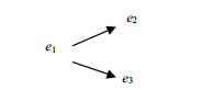
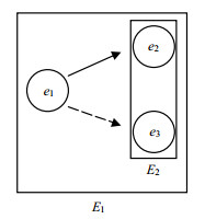
Consider two event structures E₁ and E₂ in Fig. 1, where partial ordering relation is depicted by arrow (omitting those derivable by transitivity) and conflict relation is depicted by dashed line (omitting those derivable by conflict heredity). The events of E₁ are e₁, e₂, e₃ where e₁≼e₂ and e₁# e₃. E₂ is the restriction of E₁ to {e₂, e₃}. Then, we have ${e_2}, {e_3} \in { \sim _{{E_2}}}$ Since conflict is hereditary, ${e_2}, {e_3} \notin { \sim _{{E_1}}}$.

Figure 1.  The subscript of concurrency relation

An execution of an event structure is a configuration. The notion of a configuration captures the intuition that an event can occur only after all the events that lie in its past have occurred. Formally, the definition is as follows.

Definition 6 A set is called a configuration of E iff

1) C is conflict-free in E, i.e., ∀e, e'∈C not (e#e');

2) C is left-closed in E, i.e., ∀e∈C, ∀e'∈E, e'≼e implies e'∈C;

3) |C| is finite.

The set of all configurations of E is denoted by C(E). Since ø⊆E is conflict-free and left-closed, |ø| is finite, ø∈C(E).

The semantics of event structures is typically given as partially ordered sets^[1], or labelled partially ordered sets^[12], an alternative semantical view on event structures is to consider configurations and the transitions between them.

Definition 7 A labelled transition system is a tuple (Q, Q⁰, Σ, →), where Q is a (possibly infinite) set of states; Q⁰⊆Q is a (possibly infinite) set of initial states; Σ is a (possibly infinite) set of action labels; →⊆QxΣxQ is a set of transitions.

A configuration C represents a state of E, namely, the state in which the events in C have occurred. Hence C(E) is the set of states. The initial state of E is the state where no action has been occurred yet. Hence ø is the set of initial states.

Example 2

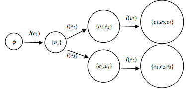
A trivial event structure E₃ is shown in Fig. 2, and the labelling function satisfies that l(e₁)=a, l(e₂)=b and l(e₃)=c. C(E₃)={ø, {e₁}, {e₁, e₂}, {e₁, e₃}, {e₁, e₂, e₃}}.

Figure 2.  Event structure E₃

Interleaving and step are respectively used in sequential nondeterministic event structures and concurrent deterministic event structures, where sequential means that every two events in the event structure are either causally related or conflicting (~_E=ø), deterministic means that the event structure does not contain any pair of conflicting events (#=ø).

In this section, we define approximate trace equivalence and approximate SF equivalence based on interleaving semantics. In the interleaving semantics, an event structure progresses through a sequence of single actions. An occurrence of a single action $a \in A \cup \tau $ leads to the state changing from configuration C₁ to configuration C₂, denoted by ${C_1}{\mathop \to \limits^a _I}{C_2}$, iff C₁⊂C₂ and $\exists $e∈E such that C₂-C₁={e}, l(e)=a. Let ${ \to _I}$ denote the set of all the leading relations. Hence:

${ \to _I}$={(C₁, a, C₂)∈C(E)×A$ \cup $τ×C(E) | ${C_1}{\mathop \to \limits^a _I}{C_2}$}

Write ε for the empty sequences of actions, a, δ for the concatenation of a∈A$ \cup $τ and δ∈(A$ \cup $τ)∞. The generalized transition ${\mathop \to \limits^\delta _I}$ is defined recursively by:

It is straightforward to show that (C(E), ø, A$ \cup $τ, ${ \to _I}$) forms a labelled transition system.

Definition 8 TS_I(E)=(C(E), ø, A$ \cup $τ, ${ \to _I}$) is called the interleaving view of E.

It is convenient to describe interleaving view by directed graphs. Each state is represented by a circle, the corresponding configuration is shown inside the circle, and a transition from one state to another is indicated by an arrow with a label.

Example 3

Consider again E₃ from Example 2, we denote the interleaving view of E₃ by Fig. 3.

Figure 3.  The interleaving view of E₃

δ∈(A∪τ)∞ is an interleaving trace of E if $\exists $C∈C(E) such that $\phi {\mathop \to \limits^\delta _I}$ C. Let T_I(E) denote the set of all interleaving traces of E. Note that repeated elements are counted only once in T_I(E).

The traditional exact interleaving trace equivalence is given as follows.

Definition 9 Two event structures E₁ and E₂ are interleaving trace equivalent, in other words, there is an interleaving trace equivalence relation between E₁ and E₂, notation E₁=_tiE₂, iff T_I(E₁)=T_I(E₂).

Definition 10 The distance between interleaving traces δ₁ and δ₂ is naturally defined as their Baire distance, δ_ti(δ₁, δ₂)=d_B(δ₁, δ₂).

Proposition 1

∀δ_j∈T_I(E_j), j=1, 2, 3

d_ti(δ₁, δ₃)≤max(d_ti(δ₁, δ₂), d_ti(δ₂, δ₃))

Proof If δ₁=δ₂ or δ₂=δ₃, then the right-hand side of the inequality is equal to the left-hand side. Hence the inequality trivially holds.

If δ₁=δ₃, then the left-hand side of the inequality is equal to 0. Hence the inequality holds.

Otherwise δ₁≠δ₂, δ₂≠δ₃ and δ₁≠δ₃. Let l∈N be the length of the longest common prefix of δ₁ and δ₂, l'∈N be the length of the longest common prefix of δ₂ and δ₃. Without loss of generality, assume l≤l', then the length of the longest common prefix of δ₁ and δ₃ is no less than l.

_ti(δ₁, δ₃)≤2^-l=max(2^-l, 2^-l')=max(d_ti(δ₁, δ₂), d_ti(δ₂, δ₃))

Hence d_ti(δ₁, δ₃)≤max(d_ti(δ₁, δ₂), d_ti(δ₂, δ₃)) holds in all cases.

The following theorem shows that the definition of d_ti is reasonable, i.e., the distance is a pseudo-metric.

Theorem 1 d_ti is a pseudo-metric on the set of interleaving traces.

Proof ∀δ_j∈T_I(E_j), j=1, 2, 3.

1) We prove that d_ti(δ₁, δ₂)=0 iff δ₁=δ₂ (identity of indiscernibles).

d_ti(δ₁, δ₂)=d_B(δ₁, δ₂)≥0, d_ti(δ₁, δ₁)=d_B(δ₁, δ₁)=0

2) We prove that d_ti(δ₁, δ₂)=d_ti(δ₂, δ₁) (symmetry).

d_ti(δ₁, δ₂)=2^-l=d_ti(δ₂, δ₁), where l=+∞ or l∈N is the length of the longest common prefix of δ₁ and δ₂.

3) We prove that d_ti(δ₁, δ₃)≤d_ti(δ₁, δ₂)+d_ti(δ₂, δ₃) (triangular inequality).

d_ti(δ₁, δ₃)≤max(d_ti(δ₁, δ₂), d_ti(δ₂, δ₃))≤d_ti(δ₁, δ₂)+d_ti(δ₂, δ₃) (Proposition 1)

Furthermore, the pseudo-metric d_ti on the set of interleaving traces naturally induces an interleaving trace distance between two event structures.

Definition 11 The interleaving trace distance between E₁ and E₂ is defined as follows:

d_ti(E₁, E₂)=d_H(T_I(E₁), T_I(E₂))

Since Hausdorff distance d_H is a pseudo-metric, the definition of d_ti is reasonable. Event structures together with the interleaving trace distance form a pseudo-metric space.

The intuitive meaning of the interleaving trace distance is as follows. For any interleaving trace of E₁ (or E₂), we can find an interleaving trace of E₂ (or E₁) such that the distance between them remains bounded by d_ti(E₁, E₂).

For clarity, we omit the configuration inside the circle in the following directed graphs.

Example 4

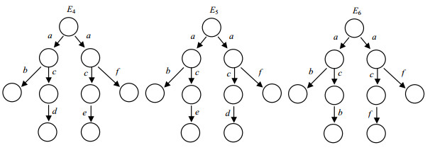
Consider the interleaving views of E₄, E₅ and E₆ in Fig. 4, where the first two directed graphs are taken from counterexample 5 in Ref.[8].

Figure 4.  A complex case

T_I(E₄)=T_I(E₅)={a, ab, ac, acd, ace, af}

T_I(E₆)={a, ab, ac, acb, acf, af}

d_ti(E₄, E₅)=0 intuitively means that for any execution of E₄ (or E₅), we can find an execution of E₅ (or E₄) such that the two executions are indistinguishable to an external observer.

d_ti(E₅, E₆)=2^-2 intuitively means that for any execution of E₅ (or E₆), we can find an execution of E₆ (or E₅) such that from the view of an external observer, the two executions share a common prefix whose length is at least 2, in other words, they are indistinguishable from the first 2 actions.

One of the great advantages of having metric structure on event structures is that the distance enables us to use quantitative approximation.

Definition 12 Two event structures E₁ and E₂ are approximate interleaving trace equivalent with the precision x≥0, in other words, there is an approximate interleaving trace relation $ \simeq _{ti}^\xi $ between E₁ and E₂, notation ${E_1} \simeq _{ti}^\xi {E_2}$, iff d_ti(E₁, E₂)≤ξ.

It is intuitive that the lower the value of ξ, the higher the degree to which $ \simeq _{ti}^\xi $ is an interleaving trace relation. It should be emphasized that two event structures are approximate interleaving trace equivalent with the precision ξ=0 is also known as they are exact interleaving trace equivalent. In other words, the traditional exact interleaving trace equivalence is a special case of approximate interleaving trace equivalence.

Theorem 2 $ \simeq _{ti}^\xi $(ξ≥0) is an equivalence relation on the set of event structures.

Proof Let E₁, E₂, E₃ be arbitrary event structures.

1) We prove that is a reflexive relation.

d_ti(E₁, E₁)=d_H(T_I(E₁), T_I(E₁))=0≤ξ, hence ${E_1} \simeq _{ti}^\xi {E_1}$

2) We prove that $ \simeq _{ti}^\xi $ is a symmetric relation. d_ti(E₁, E₂)=d_H(T_I(E₁), T_I(E₂))=d_H(T_I(E₂), T_I(E₁))=d_ti(E₂, E₁), hence ${E_1} \simeq _{ti}^\xi {E_2}$ implies that ${E_2} \simeq _{ti}^\xi {E_1}$.

3) We prove that $ \simeq _{ti}^\xi $ is a transitive relation.

Assume ${E_1} \simeq _{ti}^\xi {E_2}$ and ${E_2} \simeq _{ti}^\xi {E_3}$.

ξ≥d_ti(E₁, E₂)=d_H(T_I(E₁), T_I(E₂))=

ξ≥d_ti(E₂, E₃)=d_H(T_I(E₂), T_I(E₃))=

∀δ₁∈T_I(E₁), by Eq.(1), $\exists $δ₂∈T_I(E₂) such that d_ti(δ₁, δ₂)≤ξ. By Eq.(2), $\exists $δ₃∈T_I(E₃) such that d_ti(δ₂, δ₃)≤ξ. By Proposition 1, d_ti(δ₁, δ₃)≤max(d_ti(δ₁, δ₂), d_ti(δ₂, δ₃))≤ξ, hence:

Since this formula holds for all δ₁∈T_I(E₁),

Similarly,

d_ti(E₁, E₃)=d_H(T_I(E₁), T_I(E₃))

Example 5

Consider again the event structures in Example 4. Since d_ti(E₄, E₅) < 0.25, ${E_4} \simeq _{ti}^{0.25}{E_5}$ Since d_ti(E₅, E₆)=0.25, ${E_5} \simeq _{ti}^{0.25}{E_6}$. By Theorem 2, ${E_4} \simeq _{ti}^{0.25}{E_6}$.

The definition of singleton failure pair presented here is that of Ref.[8]. It differs from that of Ref.[13] in one important respect, the refusal set of singleton failure pair must contain one element, instead of at most one element. In our earlier work^[14], a revised version of singleton failure pair is proposed to simplify SF equivalence checking. And the RSF algorithm gains in efficiency in terms of speed than the traditional SF algorithm by reducing redundancy elements, while retaining the same information content.

The set of next interleaving actions of a configuration C is defined as follows:

N_I(C)={a∈A∪τ| $\exists $C'∈C(E) such that ${\mathop \to \limits^a _I}$ C'}

The set of possible continuations of an interleaving trace δ of E is defined as follows:

C_I(E, δ)={a∈A∪τ| $\exists $C, C'∈C(E) such that $\phi {\mathop \to \limits^a _I}$ C, C ${\mathop \to \limits^a _I}$ C'}

|δ| denotes the length of δ. If δ has infinite length, then |δ|=+∞. In order to let interleaving trace and interleaving singleton failure pair have the same form, δ is identified with a pair (δ, e) in this paper.

Definition 13 (δ, π)∈(A∪τ)∞×(A∪τ∪e) is an interleaving RSF pair of E if $\exists $C∈C(E) such that $\phi {\mathop \to \limits^\delta _I}$ C,

Let F_I(E) denote the set of all interleaving RSF pairs of E.

The traditional exact interleaving SF equivalence is given as follows.

Definition 14 Two event structures E₁ and E₂ are interleaving SF equivalent, in other words, there is an interleaving SF equivalence relation between E₁ and E₂, notation E₁=_fiE₂, iff F_I(E₁)=F_I(E₂).

Definition 15 The distance d_fi: F_I(E₁)×F_I(E₂) →[0, 1] between interleaving RSF pairs (δ₁, π₁) and (δ₂, π₂) is defined as follows:

where l is the length of the longest common prefix of δ₁ and δ₂, L is the maximum length of all interleaving traces of E₁ and E₂. l=max(|δ₁|, |δ₂|),

Hence, the definition insures that if δ₁≠δ₂, then d_fi((δ₁, π₁), (δ₂, π₂))=2^-l > 2^-L=d_fi((δ₁, π₁), (δ₂, π₁)).

Proposition 2

∀(δ_j, π_j)∈F_I(E_j) j=1, 2, 3

d_fi((δ₁, π₁), (δ₃, π₃))≤

max(d_fi((δ₁, π₁), (δ₂, π₂)), d_fi((δ₂, π₂), (δ₃, π₃)))

The proof is omitted since it is similar to the proof of Proposition 1.

Theorem 3 d_fi is a pseudo-metric on the set of interleaving RSF pairs.

The proof is omitted since it is similar to the proof of Theorem 1.

Furthermore, the pseudo-metric d_fi on the set of interleaving RSF pairs naturally induces an interleaving SF distance between two event structures.

Definition 16 The interleaving SF distance between E₁ and E₂ is defined as follows:

d_fi(E₁, E₂)=d_H(F_I(E₁), F_I(E₂))

Since Hausdorff distance d_H is a pseudo-metric, the definition of d_fi is reasonable. Event structures together with the interleaving SF distance form a pseudo-metric space.

Definition 17 Two event structures E₁ and E₂ are approximate interleaving SF equivalent with the precision ξ≥0, in other words, there is an approximate interleaving SF relation $ \simeq _{fi}^\xi $ between E₁ and E₂, notation ${E_1} \simeq _{fi}^\xi {E_2}$, iff d_fi(E₁, E₂)≤ξ.

It is intuitive that the lower the value of ξ, the higher the degree to which $ \simeq _{fi}^\xi $ is an interleaving SF relation. It should be emphasized that two event structures are approximate interleaving SF equivalent with the precision ξ=0 is also known as they are exact interleaving SF equivalent.

Theorem 4 $ \simeq _{fi}^\xi $(ξ≥0) is an equivalence relation on the set of event structures.

The proof is omitted since it is similar to the proof of Theorem 2.

In this section, we define approximate trace equivalence and approximate SF equivalence based on step semantics. In the step semantics, an event structure progresses through a sequence of steps (i.e., multi-sets of simultaneously occurring actions). The multi-set is needed, since concurrent events may have the same label.

A multi-set f:A→N is a function, ∀a∈A, f(a) is the multiplicity of a in the multi-set f.

Similarly to finitely branching labelled transition systems, which in each state has only finitely many possible ways to proceed, a multi-set f is finite iff for X={a∈A | f(a)≠ 0}, |X| is finite.

μA denotes the set of all finite multi-sets over A. Since the multi-set of simultaneously occurring actions which are all invisible (called invisible multi-set) is finite, invisible multi-set belongs to μA.

The operations on finite multi-sets are the usual operations on functions.

Definition 18 The equality operator for finite multi-sets is defined as follows:

f, g∈μA, f=g iff ∀a∈A, f(a)=g(a)

An occurrence of a finite multi-set f leads to the state changing from configuration C₁ to configuration C₂, denoted by C₁${\mathop \to \limits^f _S}$C₂, iff C₁⊂C₂ and $\exists $X⊆E such that: X is conflict-free in E; ∀e, e'∈X, e≠e', we have l(e), l(e')∈A implies (e, e')∈~_E; X defines a multi-set of actions equal to f, i.e., ∀a∈A, f(a)=|{e∈X| l(e)=a}|; X=C₂-C₁.

Let ${ \to _S}$ denote the set of all the leading relations. Hence ${ \to _S}$={(C₁, f, C₂)∈C(E)×μA×C(E)| C₁${\mathop \to \limits^f _S}$C₂}.

The generalized transition ${\mathop \to \limits^\theta _S}$ for θ∈μA∞ is defined recursively by:

It is straightforward to show that (C(E), ø, μA, ) forms a labelled transition system.

Definition 19 T_S(E)=(C(E), ø, μA, ) is called the step view of E.

Example 6

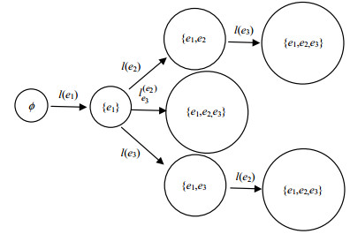
Consider again E₃ from Example 2, we denote the step view of E₃ by Fig. 5.

Figure 5.  The step view of E₃

θ∈μA∞ is a step trace of E if $\exists $C∈C(E) such that $\phi {\mathop \to \limits^\theta _S}$C. Let T_S(E) denote the set of all step traces of E.

Definition 20 Two event structures E₁ and E₂ are step trace equivalent, in other words, there is a step trace equivalence relation between E₁ and E₂, notation E₁=_tsE₂, iff T_S(E₁)=T_S(E₂).

With the help of the equality operator for finite multi-sets, we can define the distance between two step traces.

Definition 21 The distance between step traces θ₁ and θ₂ is naturally defined as their Baire distance, d_ts(θ₁, θ₂)=d_B(θ₁, θ₂).

Theorem 5 d_ts is a pseudo-metric on the set of step traces.

Definition 22 The step trace distance between E₁ and E₂ is defined as follows:

d_ts(E₁, E₂)=d_H(T_S(E₁), T_S(E₂))

Definition 23 Two event structures E₁ and E₂ are approximate step trace equivalent with the precision ξ≥0, in other words, there is an approximate step trace relation $ \simeq _{ts}^\xi $ between E₁ and E₂, notation ${E_1} \simeq _{ts}^\xi {E_2}$, iff d_ts(E₁, E₂)≤ξ.

Theorem 6 $ \simeq _{ts}^\xi $(ξ≥0) is an equivalence relation on the set of event structures.

The set of next step actions of a configuration C is defined as follows:

N_S(C)={f∈μA|$\exists $C'∈C(E) such that $C{\mathop \to \limits^f _S}$ C'}

The set of possible continuations of a step trace θ of E is defined as follows:

C_S(E, θ)={f∈μA|$\exists $C, C'∈C(E) such that $\phi {\mathop \to \limits^\theta _S}$ C, $C{\mathop \to \limits^f _S}$ C'}

Definition 24 (θ, υ)∈μA∞×μA is a step RSF pair of E if $\exists $C∈C(E) such that ${\mathop \to \limits^\theta _S}$ C,

Let F_S(E) denote the set of all step RSF pairs of E.

Definition 25 Two event structures E₁ and E₂ are step SF equivalent, notation E₁=_fsE₂, iff F_S(E₁)=F_S(E₂).

Definition 26 The distance d_fs:F_S(E₁)×F_S(E₂)→ [0, 1] between step RSF pairs (θ₁, u₁) and (θ₂, u₂) is defined as follows:

where l∈N is the length of the longest common prefix of θ₁ and θ₂, L is the maximum length of all step traces of E₁ and E₂.

Theorem 7 d_fs is a pseudo-metric on the set of step RSF pairs.

Definition 27 The step SF distance between E₁ and E₂ is defined as follows:

d_fs(E₁, E₂)=d_H(F_S(E₁), F_S(E₂))

Definition 28 Two event structures E₁ and E₂ are approximate step SF equivalent with the precision ξ≥0, in other words, there is an approximate step SF relation $ \simeq _{fs}^\xi $ between E₁ and E₂, notation ${E_1} \simeq _{fs}^\xi {E_2}$, iff d_fs(E₁, E₂)≤ξ.

Theorem 8 $ \simeq _{fs}^\xi $(ξ≥0) is an equivalence relation on the set of event structures.

Our version of Baire metric (Definition 3) is described in Ref.[11], which presented an introduction to metric semantics for programming and specification languages. In this paper, we extend the definition of Baire metric to suit the specific needs of RSF pairs (Definition 15 and Definition 26).

A metric very similar to this definition was defined by Baire^[15]. The alternative version of Baire metric was typically used to measure the similarity between strings^[16-18], but it does not support Proposition 1 and Proposition 2, which are the essential preconditions for the derivation of the transitive property of approximate equivalences.

In the past several decades, there have been many efforts to develop system approximation. Approximate trace and approximate (bi)simulation relations^[19] have been studied for transition systems^[20] and hybrid systems^[21-22] by Girard and Pappas. Their approximation is based on a metric on the set of observations, which can be any metric. However, none of their approximate relations is an equivalence relation, as they do not satisfy the transitive property. Hence their approximate relations can not be successively used, while our approximate equivalences do not have this limit. For example, ${E_1} \simeq _{ts}^\xi {E_2}, $ ${E_2} \simeq _{ts}^\xi {E_3}, \cdots, {E_{n - 1}} \simeq _{ts}^\xi {E_n}$ imply that ${E_1} \simeq _{ts}^\xi {E_n}$.

This paper proposes a generalized framework of event structures approximation by developing the notions of approximate interleaving (trace and SF) equivalence and approximate step (trace and SF) equivalence. Where interleaving and step are two discriminating views of event structures, trace semantics and SF semantics are respectively representatives of linear time semantics and branching time semantics. Note that each of these traditional exact equivalences is a special case of the corresponding approximate equivalence.

The motivation of these approximate equivalences is to define more robust relations between event structures, and to achieve a considerable complexity reduction in the approximation process.

These approximate equivalences are deduced as following. Firstly, we use Baire metric in interleaving so as to give the definition of the distance between interleaving traces (or interleaving RSF pairs). On the other hand, we regard multi-sets as functions, and define an equality operator for finite multi-sets. Therefore, we can use Baire metric in step. Then, we give the definition of the distance between step traces (or step RSF pairs). Secondly, we use Hausdorff distance d_H which is defined in Definition 4 to measure set (i.e., the set of all interleaving or step, traces or RSF pairs) distance. In other words, we define four kinds of distances on event structures. Each distance together with the event structures form a pseudo-metric space. Thirdly, these distances enable us to use quantitative approximation. We define that two event structures are approximate equivalent with the precision ξ, iff the distance between them is not greater than ξ.

The main conclusion of this paper is that these approximate equivalences satisfy the transitive property, hence they can be successively used in event structures approximation. That is to say, we can successively use these approximate equivalences to obtain a much more simplified equivalent system than an original complex system. These approximate equivalences guarantee some quality and efficiency in the specification and verification.

In our future work, we plan to develop approximate trace and SF equivalences based on partial orders.