ISSN
ISSN 


 下载:
下载:

-
Orthogonal frequency division multiplexing (OFDM), which is conducive to overcoming inter- symbol interference (ISI), has been widely used in wireless communications to achieve high spectral efficiency. The performance of coherent OFDM depends largely on the accuracy of channel estimation. Traditional channel estimation methods, such as least squares (LS), are based on the dense multipath assumption, requiring a large number of pilots to achieve satisfied performance. However, the wireless channel is widely accepted to be sparse in the delay domain[1-3], which means most channel tap coefficients corresponding to the discrete delay grids are so small that are negligible. Only the most significant taps are estimated in compressed channel estimation (CCE), in lieu of estimating all the taps as in traditional methods.
Currently, the CCE model is based upon the assumption that the wireless channel is sparse in the discrete delay grids. This means that the columns of the measurement matrix correspond to the discretized delay grids. However, the physical multipath delays are actually sparse in the continuous space[4]. The authors of Ref.[5] showed that a large deviation from the discrete grids leaded to a severe decline in the accuracy of channel estimation. This is known as the basis mismatch problem.
The authors in Ref.[6] proposed to oversample the continuous delay domain so as to alleviate the effect of basis mismatch. However, the sparse channel coefficient vector cannot be stably estimated due to the increased coherence of the over complete dictionary in the measurement matrix. Tang et al. proposed to use the atomic norm[7], which was created in the continuous space, to replace the ${l_1}$ norm so as to eliminate the effect of basis mismatch. The measurement matrices in the atomic norm method were limited to the ones with a uniform distribution. Chen and Chi proposed the use of the matrix completion method to extend the atomic norm method[8], which lifted the uniform distribution restriction on the measurement matrix. Although the atomic norm and the matrix completion methods were able to eliminate the basis mismatch problem thoroughly in theory, their solutions were related to the semi definite optimization problem, which was computationally intractable. Consequently, the above two methods were not suitable for real-time channel estimation[9-12].
In order to solve the basis mismatch problem for real-time channel estimation, many good suboptimal methods have been proposed. Nichols et al. proposed an alternating convex search algorithm, which alternatingly solved for the sparse vector and the basis mismatch vector[13]. The alternating convex search algorithm required the basis mismatch vector to be strictly convex, which was not satisfied[10-12]. The authors of Ref.[10-11] proposed that the basis mismatch could be approximated by the first order Taylor series expansion. As a result, the optimization problem for the basis mismatch vector became a convex optimization one. However, this assumption was not strictly true as the CCE model contained higher orders expansion coefficients than the first order ones.
This paper proposes a new convex optimization based alternating iteration recovery (AIR) algorithm to tackle the basis mismatch problem. The AIR algorithm aims to alternately solve for the sparse channel coefficient vector and the basis mismatch vector. Different from the aforementioned methods in the literature, the AIR algorithm is based upon an accurate CCE model, in which all the Taylor series expansion orders are included. As a result, the proposed algorithm is able to attain high performance in the channel estimation with the tractable computation.
-
Assume that one OFDM symbol contains K subcarriers, denoted as $\mathit{\boldsymbol{x}}={{[{{x}_{0}},{{x}_{1}},\cdots ,{{x}_{K-1}}]}^{\text{T}}}$. The symbol duration is T. The multipath channel model is $h(\tau ) = \sum\limits_{p = 1}^{{N_p}} {{h_p}\delta (\tau - {\tau _p})} $, where ${h_p}$ is the complex path gain of the p-th path, ${\tau _p}$ is the delay of p-th path, and ${N_p}$ is the total number of multipath. Assume that the maximum delay spread is ${\tau _{\max }}$. The multipath delay can be discretized with a sample rate ${T_s} = T/K$ to create the CCE model as follows
$${{\tau }_{n}}\in \mathcal{A}=\left\{ 0,{T}/{K}\;,2{T}/{K}\;,\cdots ,(L-1){T}/{K}\; \right\},$$ where $ L=\left\lceil {{{\tau }_{\max }}}/{{{T}_{s}}}\; \right\rceil +1$ is the total number of grids. If all the multipath delays lie exactly on these grids, i.e., ${\tau _p} \in \mathcal{A}$, the received symbol vector can be written as[14]:
$$\mathit{\boldsymbol{y}}{\rm{ = }}\mathit{\boldsymbol{XWh}}{\rm{ + }}\mathit{\boldsymbol{n}}$$ (1) where h=[h0, h1, …, hL-1] is the channel coefficient vector to be estimated, X is a diagonal matrix with vector x being its diagonal elements, n is the complex Gaussian noise vector, and W is a partial FFT matrix by selecting the first L columns of the FFT matrix, i.e.,
$$\mathit{\boldsymbol{W}} = \frac{1}{{\sqrt K }}\left[ {\begin{array}{*{20}{c}} {{w^{00}}}& \cdots &{{w^{0(L - 1)}}}\\ \vdots &{}& \vdots \\ {{w^{(K - 1)0}}}& \cdots &{{w^{(K - 1)(L - 1)}}} \end{array}} \right]$$ where ${{w}^{kl}}\triangleq \exp ({-\text{j}2\pi kl}/{K}\;)$
The above system model is based on the assumption that the multipath delays lie exactly on the discrete grid set $\mathcal{A}$, which cannot be satisfied in practical applications. The actual multipath delays are distributed on the following perturbed delay grid set
$$\begin{gathered} \mathcal{A}(\theta ) = \{ {\theta _0}, T/K + {\theta _1}, 2T/K + {\theta _2}, \cdots, \\ (L - 1)T/K + {\theta _{L - 1}}\} \\ \end{gathered} $$ Then the received symbol vector becomes
$$\mathit{\boldsymbol{y}}=\mathit{\boldsymbol{XW}}(\mathit{\boldsymbol{ \theta}}\text{ })+\mathit{\boldsymbol{n}}$$ (2) where matrix $\mathit{\boldsymbol{W}}(\mathit{\boldsymbol{ \theta}}\text{ })$ represents the basis mismatch on the delay grid, which is expressed as below:
$$\mathit{\boldsymbol{W}}(\mathit{\boldsymbol{ \theta}}\text{ })=\frac{1}{\sqrt{K}}\left[ \begin{matrix} w_{{{\theta }_{0}}}^{00} & \cdots & w_{{{\theta }_{L-1}}}^{0(L-1)} \\ \vdots & {} & \vdots \\ w_{{{\theta }_{0}}}^{(K-1)0} & \cdots & w_{{{\theta }_{L-1}}}^{(K-1)(L-1)} \\ \end{matrix} \right]$$ where $w_{{{\theta }_{l}}}^{kl}=\exp ({-j2\pi k}/{T({lT}/{K}\;+{{\theta }_{l}})}\;)$, and $\theta = {[{\theta _0}, {\theta _1}, \cdots, {\theta _{L-1}}]^{\rm{T}}}$ is the basis mismatch vector. Assume the number of pilots is P. The received pilot vector can be expressed as
$${{\mathit{\boldsymbol{y}}}_{p}}={{\mathit{\boldsymbol{X}}}_{p}}{{\mathit{\boldsymbol{W}}}_{P}}(\mathit{\boldsymbol{ \theta}}\text{ })\mathit{\boldsymbol{h}}+{{\mathit{\boldsymbol{n}}}_{p}}$$ (3) where the received pilot symbol vector ${{\mathit{\boldsymbol{y}}}_{p}}=\mathit{\boldsymbol{Sy}}$. The $P \times K$ matrix S is a selection matrix by selecting the rows indexed by the pilot positions in the eye matrix. ${{\mathit{\boldsymbol{X}}}_{p}}=\mathit{\boldsymbol{SX}}{{\mathit{\boldsymbol{S}}}^{\text{T}}}$, ${{\mathit{\boldsymbol{W}}}_{p}}(\mathit{\boldsymbol{ \theta}}\text{ })=\mathit{\boldsymbol{SW}}(\mathit{\boldsymbol{ \theta}}\text{ })$, and ${{\mathit{\boldsymbol{n}}}_{p}}=\mathit{\boldsymbol{Sn}}$. The compressed channel estimation model in (3) differs from (1) that (3) considers the basis mismatch. With the basis mismatch being taken into account, the sparse recovery problem becomes the following optimization problem[9].
$$\mathop {\min }\limits_{h,\theta } ,{{\left\| \mathit{\boldsymbol{h}} \right\|}_{1}},\;\;\;\;\;\;\;\text{s}.\text{t}.{{\left\| {{\mathit{\boldsymbol{y}}}_{p}}-{{\mathit{\boldsymbol{X}}}_{p}}{{\mathit{\boldsymbol{W}}}_{P}}(\mathit{\boldsymbol{\theta}}\text{ })\mathit{\boldsymbol{h}} \right\|}_{2}}≤\sigma $$ (4) which will solve for the sparse model ${{\mathit{\boldsymbol{W}}}_{P}}(\mathit{\boldsymbol{ \theta}}\text{ })$ and the associated channel coefficient vector h. $\sigma $ indicates the noise energy.
-
Applying the Taylor expansion to the matrix function ${{\mathit{\boldsymbol{W}}}_{P}}(\mathit{\boldsymbol{ \theta}}\text{ })$ at θ=0 gives rise to:
$${{\mathit{\boldsymbol{W}}}_{p}}(\mathit{\boldsymbol{ \theta}}\text{ })={{\mathit{\boldsymbol{W}}}_{p}}(\mathit{\pmb{0}})+\mathit{\boldsymbol{W}}_{p}^{(1)}(\mathit{\pmb{0}})\mathit{\boldsymbol{A}}(\mathit{\boldsymbol{\theta }}\text{ })+\sum\limits_{i=2}^{\infty }{\mathit{\boldsymbol{W}}_{p}^{(i)}(\mathit{\pmb{0}})\mathit{\boldsymbol{A}}{{(\mathit{\boldsymbol{ \theta}}\text{ })}^{i}}}$$ where $\mathit{\boldsymbol{A}}(\mathit{\boldsymbol{ \theta}}\text{ })=\text{diag}(\mathit{\boldsymbol{\theta }}\text{ })$, $\mathit{\boldsymbol{W}}_{p}^{(i)}=\left[ \frac{{{\partial }^{i}}{{\mathit{\boldsymbol{w}}}_{0}}}{{{\partial }^{i}}{{\mathit{\boldsymbol{ \theta}}\text{ }}_{0}}^{i}},\frac{{{\partial }^{i}}{{\mathit{\boldsymbol{w}}}_{1}}}{{{\partial }^{i}}{{\mathit{\boldsymbol{ \theta}}\text{ }}_{1}}^{i}},\cdots ,\frac{{{\partial }^{i}}{{\mathit{\boldsymbol{w}}}_{L-1}}}{{{\partial }^{i}}{{\mathit{\boldsymbol{ \theta}}\text{ }}_{L-1}}^{i}} \right]$, and wi is the (i-1)th column of matrix ${{\mathit{\boldsymbol{W}}}_{p}}(\mathit{\boldsymbol{ \theta}}\text{ })$. With the Taylor expansion, it follows from (4) that
$$\mathop {\min }\limits_{h,\theta } ,{{\left\| \mathit{\boldsymbol{h}} \right\|}_{1}},\text{s}.\text{t}.{{\left\| {{\mathit{\boldsymbol{y}}}_{p}}-{{\mathit{\boldsymbol{X}}}_{p}}\mathit{\boldsymbol{\varPhi}}\text{ }(\mathit{\boldsymbol{\theta }}\text{ })\mathit{\boldsymbol{h}}-\mathit{\boldsymbol{E}}(\mathit{\boldsymbol{h}},\mathit{\boldsymbol{ \theta}}\text{ }) \right\|}_{2}}≤\sigma $$ (5) where $\mathit{\boldsymbol{\varPhi}}(\mathit{\boldsymbol{\theta }})={{\mathit{\boldsymbol{W}}}_{p}}\mathit{\pmb{0}}+\mathit{\boldsymbol{W}}_{p}^{(1)}(\mathit{\pmb{0}})\mathit{\boldsymbol{ A}}(\mathit{\boldsymbol{\theta}})$ is a linear function of the basis mismatch θ, and the residual term $\mathit{\boldsymbol{E}}(\mathit{\boldsymbol{h}},\mathit{\boldsymbol{ \theta}}\text{ })={{\mathit{\boldsymbol{X}}}_{p}}\sum\limits_{i=2}^{\infty }{\mathit{\boldsymbol{W}}_{p}^{(i)}\mathit{\pmb{0}}\mathit{\boldsymbol{A}}{{(\mathit{\boldsymbol{\theta }}\text{ })}^{i}}\mathit{\boldsymbol{h}}}$ is a nonlinear function of θ. When the channel coefficient vector h and basis mismatch vector θ are given, $\mathit{\boldsymbol{E}}(\mathit{\boldsymbol{h}},\mathit{\boldsymbol{ \theta}}\text{ })$ can be computed as $\mathit{\boldsymbol{E}}(\mathit{\boldsymbol{h}},\mathit{\boldsymbol{\theta }}\text{ })={{\mathit{\boldsymbol{X}}}_{p}}({{\mathit{\boldsymbol{W}}}_{p}}(\mathit{\boldsymbol{ \theta}}\text{ })-\mathit{\boldsymbol{ \varPhi}}\text{ }(\mathit{\boldsymbol{ \theta}}\text{ }))\mathit{\boldsymbol{h}}$.
The optimization problem in (5) relates to two unknown vectors, i.e., h and θ. We propose the alternating iteration recovery method to estimate the two vectors. In the (i + 1)th iteration, we assume the basis mismatch vector is fixed as θ(i), which is obtained from the previous iteration. Every iteration is comprised of two stages. The first stage of the (i + 1)th iteration is to solve for h through the following optimization problem.
$$\begin{matrix} {{\mathit{\boldsymbol{h}}}_{(i+1)}}=\underset{h}{\mathop{\arg \min }}\,{{\left\| \mathit{\boldsymbol{h}} \right\|}_{1}} \\ \text{s}\text{.t}.{{\left\| {{\mathit{\boldsymbol{y}}}_{p}}-{{\mathit{\boldsymbol{X}}}_{p}}\mathit{\boldsymbol{\varPhi }}\text{ }({{\mathit{\boldsymbol{\theta }}\text{ }}_{(i)}})\mathit{\boldsymbol{h}}-\mathit{\boldsymbol{E}}({{\mathit{\boldsymbol{h}}}_{(i)}},{{\mathit{\boldsymbol{\theta }}\text{ }}_{(i)}}) \right\|}_{2}}\le {{\varepsilon }_{(i)}} \\ \end{matrix} $$ (6) where ${\varepsilon _{(i)}}$ represents the noise energy plus the residual basis mismatch in the ith iteration. The optimization problem of (6) is convex, which is also known as the basis pursuit denoising (BPDN) problem.
With the updated channel vector h(i+1), the basis mismatch vector can be estimated in the second stage of the (i + 1)th iteration as follows
$$\begin{align} & {{\mathit{\boldsymbol{\theta }}\text{ }}_{(i+1)}}=\underset{\theta }{\mathop{\arg \min }}\,{{\left\| {{\mathit{\boldsymbol{y}}}_{p}}-{{\mathit{\boldsymbol{X}}}_{p}}\mathit{\boldsymbol{ \varPhi}}\text{ }({{\mathit{\boldsymbol{\theta }}\text{ }}_{(i+1)}})\mathit{\boldsymbol{h}}-\mathit{\boldsymbol{E}}({{\mathit{\boldsymbol{h}}}_{(i+1)}},{{\mathit{\boldsymbol{\theta }}\text{ }}_{(i)}}) \right\|}_{2}} \\ & \ \ \ \ \ \ \ \ \ \ \ \ \ \ \ \ \ \ \ \text{s}\text{.t}.{{\left\| \mathit{\boldsymbol{ \theta}}\text{ } \right\|}_{\infty }}\le \beta \\ \end{align}$$ (7) where $\beta $ is an upper bound of the basis mismatch. With the updated h(i+1) and θ(i+1), the residual noise energy can be calculated as (8)
$${{\alpha }_{(i+1)}}={{\left\| {{\mathit{\boldsymbol{y}}}_{p}}-{{\mathit{\boldsymbol{X}}}_{p}}\mathit{\boldsymbol{ \varPhi}}\text{ }({{\mathit{\boldsymbol{\theta }}\text{ }}_{(i+1)}})\mathit{\boldsymbol{h}}-\mathit{\boldsymbol{E}}({{\mathit{\boldsymbol{h}}}_{(i+1)}},{{\mathit{\boldsymbol{\theta }}\text{ }}_{(i+1)}}) \right\|}_{2}}$$ (8) Two scenarios will be discussed in the following. If ${\alpha _{(i + 1)}} \geqslant \alpha $, it means that there still exists residual basis mismatch after the (i + 1)th iteration. And the residual basis mismatch should be considered as an additional noise to the Gaussian noise. If ${\alpha _{(i + 1)}} < \alpha $, it indicates that the estimated h(i+1) and θ(i+1) are "excessive matching" to (5) after the (i + 1)th iteration, which leads the iteration to be derivation from the optimal solution. In order to guarantee the convergence of the proposed AIR algorithm, the noise control term ${\varepsilon _{(i + 1)}}$ after the (i +1)th iteration should be greater than the energy of the Gaussian noise. Therefore, we update the noise control item as follows
$${\varepsilon _{(i + 1)}} = \max \left\{ {{\alpha _{(i + 1)}}, \sigma } \right\}$$ (9) where function max(:;:) returns the greater parameter in the bracket. When the iteration number i becomes large enough, the frequency response between the ith and (i−1) th iteration would be smaller than a pre-defined iteration stopping threshold TOL. The AIR algorithm then stops. The proposed AIR algorithm is described in detail in Algorithm 1.
Algorithm 1 AIR Algorithm
Inputs yp, Xp, Wp(0), Wp(1)(0), σ, β
Initialize i=0, θ(0)=0, ε(0)=σ, count, TOL
Repeat
i=i+1
Update the channel coefficient vector h(i) (6)
Update the basis mismatch vector θ(i) as per (7)
Compute the residual noise α(i)
Update ε(i) as per (8)
If i > count then
Break;
End if
Until $ \frac{{{\left\| {{\mathit{\boldsymbol{w}}}_{p}}({{\mathit{\boldsymbol{ \theta}}\text{ }}_{(i)}}){{\mathit{\boldsymbol{h}}}_{(i)}}-{{\mathit{\boldsymbol{w}}}_{p}}({{\mathit{\boldsymbol{\theta}}\text{ }}_{(i-1)}}){{\mathit{\boldsymbol{h}}}_{(i-1)}} \right\|}_{2}}}{{{\left\| {{\mathit{\boldsymbol{w}}}_{p}}({{\mathit{\boldsymbol{\theta }}\text{ }}_{(i-1)}}){{\mathit{\boldsymbol{h}}}_{(i-1)}} \right\|}_{2}}}≤\text{TOL}$
Output h, θ
-
In this section, we will provide two theorems to prove that the proposed AIR algorithm converges to the solution of (5).
Lemma 1: The output sequence triplet $\left\{ {{\mathit{\boldsymbol{h}}}_{(i)}},{{\mathit{\boldsymbol{\theta }}\text{ }}_{(i)}},{{\varepsilon }_{(i)}} \right\}$ of the proposed AIR algorithm converges to a stationary point.
Proof: As ${\alpha _{(i + 1)}} < {\varepsilon _{(i + 1)}}$, one can infer from (6) that ${{\left\| {{\mathit{\boldsymbol{h}}}_{(i+1)}} \right\|}_{1}}≤{{\left\| {{\mathit{\boldsymbol{h}}}_{(i)}} \right\|}_{1}}$, which means that ${{\left\| {{\mathit{\boldsymbol{h}}}_{(i)}} \right\|}_{1}}$, (i=0, 1, 2, …) is a monotonically decreasing sequence. $\{\mathit{\boldsymbol{\bar{h}}},\mathit{\boldsymbol{\bar{\theta}}},\bar{\varepsilon }\} $ is defined as the accumulation point of the bounded sequences $\{{{\mathit{\boldsymbol{h}}}_{(i)}},{{\mathit{\boldsymbol{\theta }}\text{ }}_{(i)}},{{\mathit{\boldsymbol{ }}\varepsilon\text{ }}_{(i)}}\} $. Then there exist sequences $\{{{\mathit{\boldsymbol{h}}}_{({{i}_{j}})}},{{\mathit{\boldsymbol{\theta }}\text{ }}_{({{i}_{j}})}},{{\mathit{\boldsymbol{ }}\varepsilon\text{ }}_{({{i}_{j}})}}\} $ (j=0, 1, 2, …), which converge to $\{\mathit{\boldsymbol{\bar{h}}},\mathit{\boldsymbol{\bar{\theta}}},\bar{\varepsilon }\} $ as subscript j tends to infinity, where h(ij) denotes a subsequence of h(i). It can be seen from (7) that ${{\left\| {{f}_{{{i}_{j}}}}(\mathit{\boldsymbol{\theta }}\text{ }) \right\|}_{2}}≥{{\left\| {{f}_{{{i}_{j}}}}({{\mathit{\boldsymbol{ \theta}}\text{ }}_{{{i}_{j}}}}) \right\|}_{2}}$, where ${{f}_{{{i}_{j}}}}({\mathit{\boldsymbol{\theta }}\text{ }})={{\mathit{\boldsymbol{y}}}_{p}}-{{\mathit{\boldsymbol{X}}}_{p}}\mathit{\boldsymbol{ \varPhi}}\text{ }({\mathit{\boldsymbol{\theta }}\text{ }}\text{ }){{\mathit{\boldsymbol{h}}}_{({{i}_{j}})}}-\mathit{\boldsymbol{E}}({{\mathit{\boldsymbol{h}}}_{({{i}_{j}})}},{{\mathit{\boldsymbol{ \theta}}\text{ }}_{({{i}_{j}}-1)}})$. The inequality is equivalent to
$$\mathit{\boldsymbol{\bar{\theta}}}=\underset{\theta }{\mathop{\arg \min }}\,\left\| {{\mathit{\boldsymbol{y}}}_{p}}-{{\mathit{\boldsymbol{X}}}_{p}}\mathit{\boldsymbol{ \varPhi}}\text{ }(\mathit{\boldsymbol{\theta }}\text{ })\mathit{\boldsymbol{\bar{h}}}-\mathit{\boldsymbol{E}}(\mathit{\boldsymbol{\bar{h}}},\mathit{\boldsymbol{ \theta}}\text{ }) \right\|$$ (10) As discussed above, the sequence $\{{{\mathit{\boldsymbol{\theta }}\text{ }}_{({{i}_{j}})}}\} $(j=1, 2, …) converges to $\{\mathit{\boldsymbol{\bar{\theta}}}\} $ as j tends to infinity. For $\forall \delta > 0$, there exists a ${j_0}$ such that when $j > {j_0}$, the inequality $\left\| {{f}_{{{i}_{j}}}}(\mathit{\boldsymbol{ \theta}}\text{ })-{{u}_{{{i}_{j}}}}(\mathit{\boldsymbol{ \theta}}\text{ }) \right\|≤\delta $ holds, where ${{u}_{{{i}_{j}}}}(\mathit{\boldsymbol{\theta }}\text{ })={{\mathit{\boldsymbol{y}}}_{p}}-{{\mathit{\boldsymbol{X}}}_{p}}\mathit{\boldsymbol{ \varPhi}}\text{ }(\mathit{\boldsymbol{\theta }}\text{ }){{\mathit{\boldsymbol{h}}}_{({{i}_{j}})}}-\mathit{\boldsymbol{E}}({{\mathit{\boldsymbol{h}}}_{({{i}_{j}})}},{{\mathit{\boldsymbol{ \theta}}\text{ }}_{({{i}_{j}})}})$. This suggests that when j is large enough, ${{u}_{{{i}_{j}}}}({\mathit{\boldsymbol{\theta }}\text{ }}\text{ })$ can be used in lieu of ${{f}_{{{i}_{j}}}}({\mathit{\boldsymbol{\theta }}\text{ }}\text{ })$ for analytical purposes. When $j \to \infty $, then $\left\| {{u}_{{{i}_{j}}}}(\mathit{\boldsymbol{\bar{\theta}}}) \right\|\to \bar{\varepsilon } $.
Define two sets ${{D}_{({{i}_{j}})}}=\left\{ \mathit{\boldsymbol{h}}\left| {{\left\| {{g}_{{{i}_{j}}}}(\mathit{\boldsymbol{h}}) \right\|}_{2}}≤{{\varepsilon }_{({{i}_{j}})}} \right. \right\}$ and $\bar{D}=\{\mathit{\boldsymbol{h}}\left| {{\left\| \bar{g}(\mathit{\boldsymbol{h}}) \right\|}_{2}}≤\sigma \right.\} $, where ${{g}_{(i)}}(\mathit{\boldsymbol{h}})={{\mathit{\boldsymbol{y}}}_{p}}-{{\mathit{\boldsymbol{X}}}_{p}}\mathit{\boldsymbol{ \varPhi}}\text{ }({{\mathit{\boldsymbol{ \theta}}\text{ }}_{(i)}})\mathit{\boldsymbol{h}}-\mathit{\boldsymbol{E}}({{\mathit{\boldsymbol{h}}}_{(i)}},{{\mathit{\boldsymbol{\theta }}\text{ }}_{(i)}})$, and $\bar{g}(\mathit{\boldsymbol{h}})={{\mathit{\boldsymbol{y}}}_{p}}-{{\mathit{\boldsymbol{X}}}_{p}}\mathit{\boldsymbol{ \varPhi}}\text{ }(\mathit{\boldsymbol{\bar{\theta}}})\mathit{\boldsymbol{h}}-\mathit{\boldsymbol{E}}(\mathit{\boldsymbol{h}},\mathit{\boldsymbol{\bar{\theta}}})$. For $\forall \mathit{\boldsymbol{h}}\in \bar{D}$, the inequality $\left\| \bar{g}(\mathit{\boldsymbol{h}}) \right\|\le \sigma \le {{\varepsilon }_{({{i}_{j}})}}$ is satisfied. We can always create a subsequence h(ij) that satisfies $\mathop {\lim }\limits_{j \to \infty }{{\mathit{\boldsymbol{h}}}_{({{i}_{j}})}}=\mathit{\boldsymbol{\bar{h}}}$. With norm inequality, the following inequality
$$\begin{matrix} \left\| {{g}_{({{i}_{j}})}}({{\mathit{\boldsymbol{h}}}_{({{i}_{j}})}}) \right\|\le \left\| \bar{g}(\mathit{\boldsymbol{h}}) \right\|+\left\| {{\mathit{\boldsymbol{X}}}_{p}} \right\|\left\| \mathit{\boldsymbol{ \varPhi}}\text{ }(\mathit{\boldsymbol{\bar{ \theta}\text{ }}})-\mathit{\boldsymbol{ \varPhi}}\text{ }({{\mathit{\boldsymbol{\theta }}\text{ }}_{({{i}_{j}})}}) \right\|\left\| {{\mathit{\boldsymbol{h}}}_{({{i}_{j}})}} \right\| \\ +\left\| {{\mathit{\boldsymbol{X}}}_{p}} \right\|\left\| \mathit{\boldsymbol{ \varPhi}}\text{ }(\mathit{\boldsymbol{\bar{\theta}}}) \right\|\left\| {{\mathit{\boldsymbol{h}}}_{{{i}_{j}}}}-\mathit{\boldsymbol{\bar{h}}} \right\|+\left\| \mathit{\boldsymbol{E}}(\mathit{\boldsymbol{h}},\mathit{\boldsymbol{\bar{\theta }\text{ }}})-\mathit{\boldsymbol{E}}({{\mathit{\boldsymbol{h}}}_{({{i}_{j}})}},{{\mathit{\boldsymbol{\theta }}\text{ }}_{({{i}_{j}})}}) \right\| \\ \end{matrix} $$ holds. Based on the definition of limit, it is easy to show when j is large enough, the created sequence $\left\{ {{\mathit{\boldsymbol{h}}}_{\left( {{\text{i}}_{\text{j}}} \right)}} \right\} $, (j=1, 2, …, ) always belongs to set ${D_{({i_j})}}$. For $\forall {D_{({i_j})}}$, the solution to (6) achieves the minimum ${l_1}$ norm, denoted as ${{\mathit{\boldsymbol{h}}}_{(j)}}\in {{D}_{({{i}_{j}})}}$. Since $\left\| {{\mathit{\boldsymbol{h}}}_{({{i}_{j}})}} \right\|\le \left\| {{\mathit{\boldsymbol{h}}}_{(j)}} \right\|$, when $j \to \infty $,$\mathit{\boldsymbol{\bar{h}}} $ has the smallest ${l_1}$ norm in set $D$, i.e.,
$$\mathit{\boldsymbol{\bar{h}}}=\underset{h}{\mathop{\arg \min }}\,\left\| \mathit{\boldsymbol{h}} \right\|,s.t.\left\| \bar{g}(\mathit{\boldsymbol{h}}) \right\|\le \bar{\varepsilon } $$ (11) Besides, ${{\left\| {{\mathit{\boldsymbol{h}}}_{(i)}} \right\|}_{1}}$is a monotonically decreasing sequence, which means the cost per iteration may either be reduced or maintained to its value. In summary, the generated sequence triplet $\{{{\mathit{\boldsymbol{h}}}_{(i)}},{{\mathit{\boldsymbol{\theta }}\text{ }}_{(i)}},{{\varepsilon }_{(i)}}\} $ converges to a stationary point of the AIR algorithm.
Lemma 2:When the iteration number is large enough, the generated sequence pair $\{{{\mathit{\boldsymbol{h}}}_{(i)}},{{\mathit{\boldsymbol{\theta }}\text{ }}_{(i)}}\} $ can be made arbitrarily close to the solution of (5).
Proof: $({{\mathit{\boldsymbol{h}}}^{*}},{{\mathit{\boldsymbol{\theta }}\text{ }}^{*}})$ is defined as the optimal solution to (5), which is also the solution to (11) with the energy of the residual noise being $\bar \varepsilon $. Assume that $({{\mathit{\boldsymbol{h}}}^{*}},{{\mathit{\boldsymbol{\theta }}\text{ }}^{*}})$ cannot satisfy (9), which means there exists a $\mathit{\boldsymbol{{\theta }\text{ }'}}$ that $\left\| q(\mathit{\boldsymbol{{ \theta}\text{ }'}}) \right\|\le \left\| q({{\mathit{\boldsymbol{\theta }}\text{ }}^{*}}) \right\|$, where $q(\mathit{\boldsymbol{ \theta}}\text{ })={{\mathit{\boldsymbol{y}}}_{p}}-{{\mathit{\boldsymbol{X}}}_{p}}\mathit{\boldsymbol{ \varPhi}}\text{ }(\mathit{\boldsymbol{\theta }}\text{ }){{\mathit{\boldsymbol{h}}}^{*}}-\mathit{\boldsymbol{E}}({{\mathit{\boldsymbol{h}}}^{*}},\mathit{\boldsymbol{\theta }}\text{ })$. Denote by h' as the solution to
$$\underset{h}{\mathop{\arg \min }}\,\left\| \mathit{\boldsymbol{h}} \right\|,s.t.\left\| p(\mathit{\boldsymbol{h}}) \right\|\le \bar{\varepsilon } $$ (12) where $p(\mathit{\boldsymbol{h}})={{\mathit{\boldsymbol{y}}}_{p}}-{{\mathit{\boldsymbol{X}}}_{p}}\mathit{\boldsymbol{ }}\varPhi\text{ }(\mathit{\boldsymbol{{ }\theta\text{ }'}})\mathit{\boldsymbol{h}}-\mathit{\boldsymbol{E}}(\mathit{\boldsymbol{h}},\mathit{\boldsymbol{{ }\theta\text{ }'}})$. Since $p(\mathit{\boldsymbol{{h}'}})\le \bar{\varepsilon } $, $(\mathit{\boldsymbol{{h}'}},\mathit{\boldsymbol{{ }\theta\text{ }'}})$ is also a feasible solution to (5). Because $\left\| {\mathit{\boldsymbol{{h}'}}} \right\|\le \left\| {{\mathit{\boldsymbol{h}}}^{*}} \right\|$, this contradicts the fact that $({{\mathit{\boldsymbol{h}}}^{*}},{{\mathit{\boldsymbol{ \theta}}\text{ }}^{*}})$is the optimal solution. Hence, the optimal solution $({{\mathit{\boldsymbol{h}}}^{*}},{{\mathit{\boldsymbol{ \theta}}\text{ }}^{*}})$ satisfies (7). In summary, the optimal solution to (5) is a stationary point of the proposed AIR algorithm. According to Lemma 1, it can be concluded that when the iteration number is large enough, the generated sequence pair $({{\mathit{\boldsymbol{h}}}_{(i)}},{{\mathit{\boldsymbol{\theta }}\text{ }}_{(i)}})$ can be made arbitrarily close to the solution of (5).
-
In this section, we will present simulation results to validate the proposed AIR algorithm. In our simulations, the multipath delay perturbations are assumed to be distributed uniformly in $[ - \beta ,\beta ]$. The maximum delay spread ${\tau _{\max }}$ is chosen to be T=4. The complex gains of the multipaths are assumed to obey a Rayleigh distribution with an average power decreasing exponentially with the delay. The total number of subcarriers in one OFDM is 512, and the number of pilots is assumed to be 40.
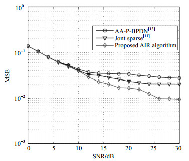
Two comparative algorithms are chosen from [11] and [13], which are suitable for the real-time channel estimation. All the algorithms are based on convex optimization. Fig. 1 plots the mean square error (MSE) versus the signal-to-noise (SNR) for these comparative algorithms. The sparsity of channel coefficients is set to be 10, and the off-grid bound is set to be 0.5. As can be seen from Fig. 1, the proposed AIR algorithm performs better in the sense of the MSE than the other two comparative algorithms. This is because the proposed AIR algorithm is based upon an accurate signal model than the other algorithms. The inaccurate model is equivalent to introducing additional noise. It also can be seen that the MSE performances of these algorithms are improved with an increase in SNR. However, their MSE performances saturate when the SNR is large enough, e.g., 25 dB. This is because the basis mismatch effect cannot be completely eliminated even at high SNRs. When the SNR is large enough, the residual noise energy is equivalent to the energy of residual basis mismatch.

Figure 1. MSE performance comparisons among algorithms with different SNRs.
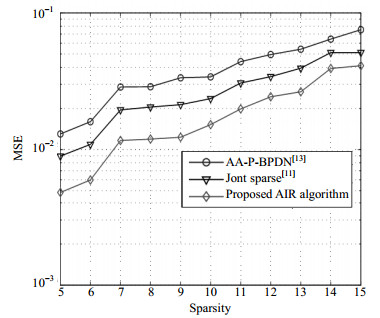
Fig.2 plots the MSE performances versus sparsity for the comparative algorithms. The SNR and the off-grid bound are set to be 20 dB and 0.5, respectively. The sparsity is defined as the number of non-zero elements in the channel coefficient vector $\mathit{\boldsymbol{h}}$, i.e., ${\left\| \mathit{\boldsymbol{h}} \right\|_0}$. It can be seen that the proposed AIR algorithm achieves better estimation performance compared with other algorithms. When the channel becomes more sparse, the MSE performances of the algorithms deteriorate.

Figure 2. MSE performance comparisons among algorithms with different sparsity
Fig. 3 shows the MSE performance versus the off-grid bound. As can be seen from the figure, the estimation performances of the three comparative algorithms are identical, when the off-grid bound is zero. However, the proposed AIR algorithm performs the best when the off-grid bound is present, although the performances of all the algorithms deteriorate with the increase of the off-grid bound. This is because the energy of the residual noise becomes large with an increase in the off-grid bound.

Figure 3. MSE performance comparisons among algorithms with basis mismatch.
-
The multipath delays in a wireless channel are actually sparse in the continuous space. The so-called basis mismatch phenomenon will cause the channel estimation performance to degrade. We propose a new convex optimization based alternating iteration recovery algorithm to reduce the effect of basis mismatch. The proposed AIR algorithm alternates to solve for the sparse channel coefficient vector and the basis mismatch vector. The algorithm uses an accurate optimization model while maintaining the convexity property at the same time. As a result, the AIR algorithm is able to obtain superior channel estimation performance.
A New Alternating Iteration Recovery Algorithm for Compressed Channel Estimation with Basis Mismatch
-
摘要: 针对压缩信道估计基失配问题进行研究,基失配本质是无线信道多径时延并不是分布在预先划分好的离散网格点上,而是呈连续分布,目前的压缩信道估计均是基于离散网格点分布假设建立估计模型,实际物理多径时延相对于离散网格点的偏差会带来信道估计性能的下降。针对该问题,提出了一种新的迭代凸优化信道估计算法,该算法交替迭代求解稀疏信道向量和基失配向量,并且每一步迭代过程均为凸优化问题。仿真分析结果表明算法在保证收敛性的同时,取得相比于比较算法更好的性能。Abstract: This paper tackles the well-known problem of basis mismatch in compressed channel estimation for wireless channels. The basis mismatch problem is caused by the fact that multipath delays exist in the continuous space, not exactly on the discretized grid. Any deviation from the grid points leads to performance degradation in channel estimation. This problem is known as the basis mismatch problem in the compressed channel estimation. In the paper, we propose a new convex optimization based alternating iteration recovery (AIR) algorithm to alternately solve the sparse channel coefficient vector and the basis mismatch vector. The optimization problems in each stage of the iterations are convex. The results show that the proposed AIR algorithm achieves better estimation accuracy compared with the comparative algorithms.
-
Key words:
- alternating iteration recovery /
- basis mismatch /
- channel estimation /
- convex /
- multipath channel
-
[1] BAJWA W U, HAUPT J, SAYEED A M, et al. Compressed channel sensing:a new approach to estimating sparse multipath channels[J]. Proceedings of the IEEE, 2010, 98(6):1058-1076. doi: 10.1109/JPROC.2010.2042415 [2] TAUBOCK G, HLAWATSCH F, EIWEN D, et al. Compressive estimation of doubly selective channels in multicarrier systems:Leakage effects and sparsityenhancing processing[J]. IEEE Journal of Selected Topics in Signal Processing, 2010, 4(2):255-271. doi: 10.1109/JSTSP.2010.2042410 [3] MENG J, YIN W, LI Y, et al. Compressive sensing based high-resolution channel estimation for OFDM system[J]. IEEE Journal of Selected Topics in Signal Processing, 2012, 16(1):15-25. [4] BERGER C R, ZHOU S, PREISIG J C, et al. Sparse channel estimation for multicarrier underwater acoustic communication:From subspace methods to compressed sensing[J]. IEEE Transactions on Signal Processing, 2010, 58(3):1708-1721. doi: 10.1109/TSP.2009.2038424 [5] CHI Y, SCHARF L L, PEZESHKI A, et al. Sensitivity to basis mismatch in compressed sensing[J]. IEEE Transactions on Signal Processing, 2011, 59(5):2182-2195. doi: 10.1109/TSP.2011.2112650 [6] QU F, NIE X, XU W. A two-stage approach for the estimation of doubly spread acoustic channels[J]. IEEE Journal of Oceanic Engineering, 2015, 40(1):131-143. doi: 10.1109/JOE.2014.2307194 [7] TANG G, BHASKAR B N, SHAH P, et al. Compressed sensing off the grid[J]. IEEE Transactions on Information Theory, 2013, 59(11):7465-7490. doi: 10.1109/TIT.2013.2277451 [8] CHEN Y, CHI Y. Robust spectral compressed sensing via structured matrix completion[J]. IEEE Transactions on Information Theory, 2014, 60(10):6576-6601. doi: 10.1109/TIT.2014.2343623 [9] CANDES E J, GRANDA C F. Towards a mathematical theory of super-resolution[J]. Communications on Pure Applied Mathematics, 2014, 67(6):906-956. doi: 10.1002/cpa.v67.6 [10] TAN Z, YANG P, NEHORAI A. Joint sparse recovery method for compressed sensing with structured dictionary mismatches[J]. IEEE Transactions on Signal Processing, 2014, 62(19):4997-5008. doi: 10.1109/TSP.2014.2343940 [11] YANG Z, XIE L. Exact joint sparse frequency recovery via optimization methods[J]. IEEE Transactions on Signal Processing, 2016, 64(19):5145-5157. doi: 10.1109/TSP.2016.2576422 [12] QING X, HU G, WANG X. Robust compressed sensing with bounded and structured uncertainties[J]. IET Signal Processing, 2014, 8(7):783-791. doi: 10.1049/iet-spr.2013.0260 [13] NICHOLS J M, OH A K, WILLET R M. Reducing basis mismatch in harmonic signal recovery via alternating convex search[J]. IEEE Signal Processing Letters, 2014, 21(8):1007-1011. doi: 10.1109/LSP.2014.2322444 [14] LIU Y, TAN Z, HU H, et al. Channel estimation for OFDM[J]. IEEE Communications Surveys & Tutorials, 2014, 16(4):1891-1908. -

 点击查看大图
图(3)
计量
- 文章访问数: 3473
- HTML全文浏览量: 1157
- PDF下载量: 84
- 被引次数: 0