The following subsections will present basic definitions used in the kinematic models.

Before an introduction of the dual quaternions, let us consider ordinary quaternions. A quaternion may be defined as

where ${q_0}$, ${q_1}$, ${q_2}$ and ${q_3}$ are real numbers, whereas $\tilde \imath ,\tilde \jmath $ and $\tilde k$ are hipercomplex numbers, having properties

The scalar component of quaternion $\tilde q$ is defined as and the vector component as , where the superscript ${\text{T}}$ denotes transposition.

Let us describe a quaternion by a vector, e.g.,

Multiplication of quaternion $\tilde q$ by a scalar $s$ gives

Addition of quaternion $\tilde g = {g_0} + {g_1}\tilde \imath + {g_2}\tilde \jmath + {g_3}\tilde k$ to quaternion $\tilde h = {h_0} + {h_1}\tilde \imath + {h_2}\tilde \jmath + {h_3}\tilde k$ acts in a component-wise way

The product of quaternions $\tilde g$ and $\tilde h$ is

Assume that ${ {\mathbb{R}}^{m \times n}}$ is the set of all $m \times n$ matrices of real numbers. Consider the matrix

where ${{\mathit{\boldsymbol{g}}}_{11}} \in \mathbb{R}$, ${{\mathit{\boldsymbol{g}}}_{12}} \in {\mathbb{R}^{1 \times 3}}$, ${{\mathit{\boldsymbol{g}}}_{21}} \in {\mathbb{R}^{3 \times 1}}$ and ${{\mathit{\boldsymbol{g}}}_{22}} \in {\mathbb{R}^{3 \times 3}}$. Now, let us define the product of matrix ${\mathit{\boldsymbol{g}}}$ and quaternion $\tilde h$:

Note that the above product is a quaternion.

The conjugate of quaternion $\tilde q$ is defined as

The quaternion norm $\left\| {\tilde q} \right\|$ can be defined by

A quaternion $\tilde q$ with the norm $\left\| {\tilde q} \right\| = \tilde 1$ is called a unit quaternion, assuming that $\tilde 1$ is the quaternion identity defined as

Let ${{\mathit{\boldsymbol{{\hat a}}}}}$ be a unit vector specifying an axis of rotation. Let $\varphi $ be an angle of rotation about axis ${{\mathit{\boldsymbol{{\hat a}}}}}$. Then the rotation may be described by a unit quaternion

Assume that roll ${\psi _1}$, pitch ${\psi _2}$ and yaw ${\psi _3}$ describe a rotation of frame $\{ B\} $ about fixed axes $\{ {{{\mathit{\boldsymbol{\hat a}}}}_{1A}},{{{\mathit{\boldsymbol{\hat a}}}}_{2A}},{{{\mathit{\boldsymbol{\hat a}}}}_{3A}}\} $ of frame $\{ A\} $. This set of angles can be converted to an equivalent unit quaternion, representing the rotation

Let the origin of frame $\{ H\} $ coincide with the origin of frame $\{ G\} $. Suppose that $\{ H\} $is rotated relative to $\{ G\} $ by roll, pitch and yaw expressed by an orientation vector . Let be a vector expressed in $\{ H\} $. We can convert $^H{{\mathit{\boldsymbol{a}}}}$ into quaternion using

Let $_H^G\tilde r$ be an unit quaternion, which maps the quaternion $^H\tilde a$ written with respect to frame $\{ H\} $ into quaternion $^G\tilde a$ expressed in frame $\{ G\} $. Then,

The unit quaternion ${}_H^G\tilde r$, which represents rotation of frame $\{ H\} $ relative to $\{ G\} $, can be found using (13) and $^G{{{\mathit{\boldsymbol{\psi }}}}_H}$. The inverse transformation to the one described by (15) can be obtained using ${}_G^H\tilde r = {}_H^G{\tilde r^*}$:

A dual number is defined as

where ${n_r}$ is the real part, ${n_d}$ is the dual part, and ${E^2} = 0$ but $E \ne 0$. The objects ${n_r}$ and ${n_d}$ can be real numbers, vectors, quaternions etc.; or more generally, elements of an algebraic field. The real part of a dual number $D$ may be denoted by and the dual part by .

The multiplication of a dual number $D$ by a real number $s$ results in

Assume that dual numbers $G$ and $H$ are such that $G = {g_r} + E{g_d}$ and $H = {h_r} + E{h_d}$, then their sum is

and their product is

A dual quaternion $Q$ is defined as

which is a dual number, where both the real part ${\tilde q_r}$ and the dual part ${\tilde q_d}$ are ordinary quaternions.

The addition of dual quaternions and multiplication of dual quaternion by a scalar or another dual quaternion are under the same rules as operations on dual numbers described in Section 1.3. According to (20), the product of dual matrix $G = {{\mathit{\boldsymbol{g}}}_r} + E{{\mathit{\boldsymbol{g}}}_d}$ and dual quaternion $H = {\tilde h_r} + E{\tilde h_d}$ is

where ${{\mathit{\boldsymbol{g}}}_r} \in {\mathbb{R}^{4 \times 4}}$, ${{\mathit{\boldsymbol{g}}}_d} \in {\mathbb{R}^{4 \times 4}}$ and the product of a $4 \times 4$ matrix and an ordinary quaternion is given by (8). In the special case, ${{\mathit{\boldsymbol{g}}}_r} = {\mathit{\boldsymbol{g}}}\frac{{\text{d}}}{{{\text{d}}E}}$, where is a differential operator [10], and ${\mathit{\boldsymbol{g}}} \in {\mathbb{R}^{4 \times 4}}$, we may write

In the both cases, the product is a dual quaternion.

Suppose that

then the transformation $\bar C$ of a dual quaternion $Q$ is defined as

Let ${{\mathit{\boldsymbol{Q}}}}$ be $m \times n$ matrix of dual quaternions such that

then transformation is defined as

A dual quaternion $Q$ indeed has three conjugates. In this study we will use one of them

The dual quaternion norm $\left\| Q \right\|$ is defined as

The dual quaternion identity is

A dual quaternion $Q$ such that $\left\| Q \right\| = I$ is called a unit dual quaternion.

Both the rotation and translation of a frame $\{ H\} $ relative to a frame $\{ G\} $ can be represented by the unit dual quaternion

wherein ${}_H^G\tilde r$ is an unit quaternion representing rotation, which can be found by using (13) and

Equation (32) is a quaternion which represents translation of $\left\{ H \right\}$ relative to $\left\{ G \right\}$ by a vector ${}^G{{{\mathit{\boldsymbol{p}}}}_H}$. Given $_H^GT$, we may find

Let $_G^HT$ represent the inverse transformation to the one described by $_H^GT$, then

A unit dual quaternion, which describes only frame rotation by an angle $\varphi $ about an axis represented by an unit vector ${{\mathit{\boldsymbol{\hat a}}}}$, may be expressed as

An unit dual quaternion, which represents only a translation along ${{\mathit{\boldsymbol{\hat a}}}}$ by a distance $p$, is given by

Let ${}^H{{\mathit{\boldsymbol{a}}}} \in {\mathbb{R}^{3 \times 1}}$ and ${}^H{{\mathit{\boldsymbol{b}}}} \in {\mathbb{R}^{3 \times 1}}$ be free vectors written with respect to a frame $\{ H\} $ and

then we may map this dual quaternion into

which is written in terms of frame $\{ G\} $, using the transformation

where $_H^GT$ is a unit dual quaternion which describes a pose (position and orientation) of $\{ H\} $ with respect to $\{ G\} $.

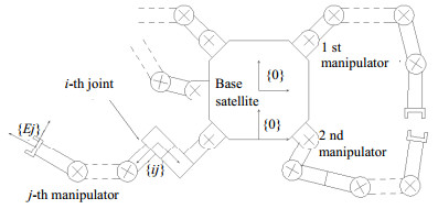
This section presents direct and inverse velocity kinematics of a multi-arm free-floating robot. An example of the robot architecture with basic symbol definitions is depicted in Fig. 1. In the case of vectors denoting a position or velocity relative to an inertial frame $\{ N\} $, superscripts and subscripts $N$ will be omitted.

Figure 1.  An example of the robot architecture

Assume that frame $\{ 0\} $ is arbitrarily affixed to the base satellite. Let be a vector pointing the origin of $\{ 0\} $, and be the orientation of $\{ 0\} $, wherein ${\psi _{10}}$ is roll, ${\psi _{20}}$ is pitch and ${\psi _{30}}$ is yaw; also let both ${{{\mathit{\boldsymbol{p}}}}_0}$ and ${{{\mathit{\boldsymbol{\psi }}}}_0}$ be expressed in the inertial frame $\{ N\} $. We define

Assume that unit dual quaternion ${}_0^NT$ represents position and orientation of the base satellite frame $\left\{ 0 \right\}$ relative to the inertial reference frame $\{ N\} $ and

where the quaternion representing translation of frame $\{ 0\} $ relative to $\{ N\} $ is given by

and the quaternion ${}_0^N\tilde r$ representing rotation of $\{ 0\} $ relative to $\{ N\} $ may be found using (13) and ${{{\mathit{\boldsymbol{\psi }}}}_0}$.

Suppose that frame $\{ ij\} $ is fixed to $i{\text{ - th}}$ joint of $j{\text{ - th}}$ manipulator (see Fig. 1) and defined by unit vector triad $\{ {{{\mathit{\boldsymbol{\hat a}}}}_{1ij}},{{{\mathit{\boldsymbol{\hat a}}}}_{2ij}},{{{\mathit{\boldsymbol{\hat a}}}}_{3ij}}\} $. Further, assume that ${{{\mathit{\boldsymbol{\hat a}}}}_{3ij}}$ is coincident with the axis of $i{\text{ - th}}$ joint of $j{\text{ - th}}$ manipulator and ${{{\mathit{\boldsymbol{\hat a}}}}_{1ij}}$ is coincident with mutually perpendicular line connecting the axes of $i{\text{ - th}}$and $(i + 1){\text{ - th}}$ joints of $j{\text{ - th}}$ manipulator. Such an assignment of frames is fully consistent with the convention used in [11]. Let us assume that unit dual quaternion ${}_{ij}^{i - 1|j}T$ describes orientation of $\{ ij\} $ relative to frame $\{ i - 1|j\} $. Then, ${}_{ij}^{i - 1|j}T$ can be formulated as a function of four Denavit-Hartenberg parameters: link length ${l_{i - 1|j}}$, link twist angle ${\alpha _{i - 1|j}}$, joint offset ${d_{ij}}$ and joint angle ${\theta _{ij}}$:

where and can be found by using (35) and (36), respectively.

A pose of $i{\text{ - th}}$ joint of $j{\text{ - th}}$ manipulator relative to $w{\text{ - th}}$ joint of the same manipulator, for $w < i$, is given by

where ${}_{kj}^{k - 1|j}T$ can be found by using (43). If $w = i$, then ${}_{ij}^{wj}T = I$, given by (30). For $w = 0$, we have ${}_{ij}^{wj}T = {}_{ij}^0T$. A pose of $i{\text{ - th}}$ joint of $j{\text{ - th}}$ manipulator, expressed in the inertial frame $\{ N\} $ is given by

Let ${n_j}$ denote the number of joints of $j{\text{ - th}}$ manipulator and frame $\{ Ej\} $ be rigidly fixed to the end-effector of this manipulator. Assume that ${}_{Ej}^{{n_j}j}T$ is a unit dual quaternion, describing pose of $\{ Ej\} $ in the frame of the last joint $\{ {n_j}j\} $ (wrist frame), then the direct kinematics of $j{\text{ - th}}$ end-effector may be written as

where ${}_{Ej}^NT$ describes the pose of the end-effector with respect to the inertial frame $\{ N\} $ and ${}_{{n_j}j}^NT$ can be found by using (45).

Both the linear velocity ${}^{ij}{{\mathit{\boldsymbol{ \boldsymbol{v} }}}_{ij}}$ as well as the angular velocity ${}^{ij}{{\mathit{\boldsymbol{ \boldsymbol{\omega } }}}_{ij}}$ of $i{\text{ - th}}$ joint of $j{\text{ - th}}$ manipulator, relative to the inertial frame $\{ N\} $, may be expressed in the joint frame $\{ ij\} $ itself by a dual quaternion

Define a $\zeta \times 1$ joint vector for $j{\text{ - th}}$ manipulator,

where ${\nu _{wj}} = {d_{wj}}$ if $w{\text{ - th}}$ joint is prismatic and ${\nu _{wj}} = {\theta _{wj}}$ if the joint is revolute.

Suppose that the frame $\{ X\} $ is rigidly fixed relative to ${\zeta _X}{\text{ - th}}$ body of $j{\text{ - th}}$ manipulator and the dual velocity of $\{ X\} $ written in this frame itself and relative to the inertial frame $\{ N\} $ is given by

where ${}^X{{{\mathit{\boldsymbol{J}}}}_{X\left\langle 0 \right\rangle }}$ is a $1 \times 6$ Jacobian matrix of dual quaternions, which is related to the velocity of $\{ X\} $ caused by the motion of the base satellite,

and ${}^X{{{\mathit{\boldsymbol{J}}}}_{X\langle M\rangle }}$ is a $1 \times {\zeta _X}$ Jacobian matrix of dual quaternions, which is related to the velocity of $\{ X\} $ caused by motion of the joints of j-th manipulator

Now, suppose that frame $\{ Y\} $ is fixed relative to the ${\zeta _Y}$-th body of j-th manipulator, whereas ${\zeta _Y} \geqslant {\zeta _X}$ and ${\zeta _Y} \geqslant 1$. The dual velocity of $\{ Y\} $, expressed in frame $\{ Z\} $ and relative to $\{ N\} $ may be found by

where

wherein, for $c \in \left\{ {1,2,3} \right\}$,

whereas, ${}^X{{{\mathit{\boldsymbol{\hat a}}}}_S}$ is a unit vector directing the axis of rotation of the base satellite relative to the inertial frame $\{ N\} $ and ${}^X{{{\mathit{\boldsymbol{p}}}}_Y}$ is a vector pointing the origin of frame $\{ Y\} $. Note that both ${}^X{{{\mathit{\boldsymbol{\hat a}}}}_S}$ and ${}^X{{{\mathit{\boldsymbol{p}}}}_Y}$ are written in the frame $\{ X\} $. Using the assumed way of orientation description, the subscript $S$ may be replaced with $cN$. Meanwhile,

For $w \in \{ 1, \cdots ,{\zeta _Y}\} $, if w-th joint is prismatic, then

If $w$-th joint is revolute, then

where ${}^X{{{\mathit{\boldsymbol{\hat a}}}}_L}$ is an unit vector directing the axis of $w{\text{ - th}}$ joint and expressed in frame $\{ X\} $. Using the assumed way of joint frames assignment, the subscript $L$ may be replaced with $3wj$.

For the dual velocity equations, we need to obtain $c{\text{ - th}}$ axis of rotation of the base satellite relative to an inertial frame, expressed in the base frame, for $c \in \{ 1,2,3\} $. This axis is described by a unit vector ${}^0{{{\mathit{\boldsymbol{\hat a}}}}_{cN}}$, directing the $c{\text{ - th}}$ axis of the inertial frame $\{ N\} $ and expressed in the main base frame $\{ 0\} $, such that

where ${{{\mathit{\boldsymbol{\hat a}}}}_{cN}}$ is the $c{\text{ - th}}$ axis of $\{ N\} $ written in this frame itself and ${}_N^0\tilde r = {}_0^N{\tilde r^*}$. In (54) and (55), for $X = 0$ we have and ${}^0{J_{0\left\langle {\psi c0} \right\rangle }} = $ , respectively.

For $w \leqslant i$, let . If $X = ij$ and $w = 0$, then ${}_{wj}^{ij}\tilde r = {}_0^X\tilde r$, we may obtain the unit vector

According to the assumed convention of joint frames assignment, we have .

In (57) and (58), for $X = wj$, we have

respectively.

For $X = ij$, we may find the unit quaternion directing the axis of $w{\text{ - th}}$ joint of $j$-th manipulator, expressed in the frame of $i{\text{ - th}}$ joint of the same manipulator,

In (55) and (58), if $X = wj$ and $Y = ij$, then

This includes the case of $w = 0$.

The velocity of an arbitrary robot component can be calculated using Jacobian matrix elements given by (54), (55), (57) and (58); whereas the symbols used in these equations are substituted according to Table 1, for prismatic joints the symbol $\nu $ is replaced with $d$ and in the case of a revolute joint $\nu $ is replaced with $\theta $. A dual quaternion ${}_X^ZT$ for the transformation ${}_X^Z{T_\varrho }$ can be calculated using methods from Section 2.1. However, some Jacobian elements, e.g., ${J_{Ej\langle pc0\rangle }}$, ${J_{Ej\langle \psi c0\rangle }}$ and ${J_{Ej\langle \nu wj\rangle }}$ in the end-effector's velocity equation, can be calculated after ${}^{{n_j}j}{J_{{n_j}j\langle pc0\rangle }}$, ${}^{{n_j}j}{J_{{n_j}j\left\langle {\psi c0} \right\rangle }}$ and ${}^{{n_j}j}{J_{{n_j}j\langle \nu wj\rangle }}$ are found first. Let

where ${{\mathit{\boldsymbol{ \boldsymbol{\varTheta} }}}_j} = {{\mathit{\boldsymbol{ \boldsymbol{\varTheta} }}}_{{n_j}j}}$ and ${n_M}$ is the number of manipulators. Assuming that ${{\mathit{\pmb{0}}}_{1 \times {n_j}}}$ is a row vector of zero dual quaternions, the direct velocity kinematics of all end-effectors of a multi-arm free floating robot can be expressed as

The inverse velocity kinematics of a free floating robot need to be solved with consideration of the system dynamical parameters.

Let frame $\{ B\} $ be rigidly fixed to a body $B$ and origin of frame $\{ CB\} $ be coincident with the center of mass of $B$. Let${m_B}$ be the mass of body $B$ and ${}^{CB}{I_{ccB}}$ be the mass moment of inertia of $B$, where $c \in \{ 1,2,3\} $ is an axis number. Now define the dual inertia matrix of the body $B$ relative to $\{ CB\} $ as

where $\frac{{\text{d}}}{{{\text{d}}E}}$ is a differential operator invented in [10].

Define a matrix of dual quaternions

where for $\nu \in \{ p,\psi \} $ and $B \in \{ 0,ij,Ej\} $,

Note that the products of the dual matrices and Jacobian elements are defined according to (23).

Also, define

where, for $w \in \{ 1, \cdots ,{n_j}\} $, if $w{\text{ - th}}$ joint is prismatic then the symbols $\nu w$ are replaced by $dw$, if the joint is revolute then $\nu w$ are replaced by $\theta w$, and

Note that the Jacobian elements can be calculated by using (54), (55), (57) and (58), whereas the symbols in these equations are substituted according to Table 1. Now, both the linear and angular momentum of the robot can be expressed by a dual momentum

where

With the knowledge on initial dual momentum $M$ and joint velocities ${\mathit{\boldsymbol{ \boldsymbol{\dot \varTheta} }}}$, we may employ (72) to find

where the transformations $\bar C$ and $\bar M$ are given by (25) and (27), respectively, and the superscript $^{ - 1}$ denotes an inverted matrix. Substituting (74) into (66), the fowling equation is obtained:

where ${{{\mathit{\boldsymbol{J}}}}_\mathcal{G}}$ is ${n_M} \times {n_M}$ generalized Jacobian matrix in the dual quaternion domain.

In the case where each manipulator has exactly six joints, we may solve the inverse velocity kinematics by

However, in a practical application, inversion of the Jacobian in the above equation is not feasible, especially when ${n_M} > 1$. It is recommended to obtain $\mathop {\mathit{\boldsymbol{ \boldsymbol{\varTheta} }}}\limits^{\bf{.}} $ by an employment of a linear equations solver.

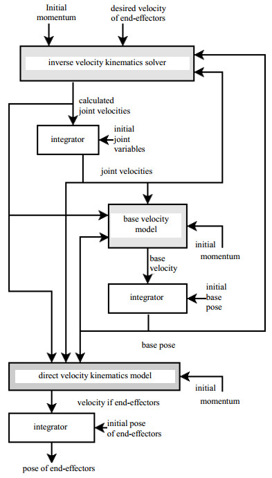
To verify the obtained kinematic models, a computer simulation of kinematic control process is executed. The process is illustrated in Fig. 2. In this process, the inverse velocity kinematics solver given by (76) calculates joint variables rates, which are fed into the direct velocity kinematics model (75). Then we may analyze the error between the desired and the obtained velocity of end-effectors. The kinematic models require the current base pose, hence the model of base velocity (74) is introduced. A robot with two different manipulators has been considered. Both the manipulators have six degrees of freedom and identical end-effectors.

Figure 2.  Simulated control process

The control system has been implemented as a library in C++ language, with an application of the Eigen library [12] for solution of sets of linear equations. 32-bit representation of real numbers has been used.

Data such as parameters of the simulated robot base, parameters of the links and end-effectors of the robot, initial conditions, and desired velocity of end-effectors, are given in [13].

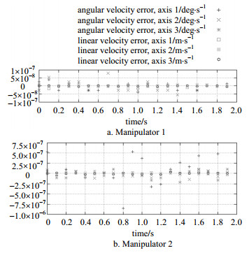
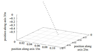
The errors between the desired and the obtained velocities are shown in Fig. 3. For some example, the calculated joint velocities result in position of manipulator 2 end-effector depicted in Fig. 4. Note that the position is given relative to the initial poses.

Figure 3.  Velocity error

Figure 4.  Position of manipulator 2 end-effector

This paper presents methods for solution of the direct and inverse velocity kinematics of a free floating robot. The methods are based on the concept of generalized Jacobian matrix, which enables a consideration of the dynamical interactions between manipulators and the base satellite.

The presented methods may be applied to robots with an arbitrary number of manipulators, where the manipulators may have an arbitrary order of prismatic and revolute joints. The kinematic models are functions of parameters widely used in robotics (such as Denavit–Hartenberg parameters). The methods may be used for manipulators with nonconventional joint twist angles.

However, approaches based on the generalized Jacobians are sensitive to dynamical singularities. Therefore, they require a supervisory system for an intelligent trajectory via-points planning.

Computational efficiency, especially important in the systems with complicated kinematics, has been improved by an application of dual quaternions for body pose representation.

The correctness of the methods is demonstrated by a computer simulation, with consideration of practical robot parameters. The used simulation software enables observation of many important parameters, such as end-effectors' pose, velocity or the base displacement, which is useful in the design of a practical system.