 ISSN
ISSN 


-
With the development of complex network research, many more real complex systems have been described as complex network[1-5]. Link prediction aims to predict the likelihood that a link exists between two endpoints in complex networks[6]. Predicting missing links plays an important role in discovering the unknown connections in protein-protein interaction networks[7], forecasting the future relationships in online social networks[8], and identifying spurious flights in air transportation networks[9].
Based on evolution mechanisms of complex networks, a lot of link prediction methods have been proposed. Among these methods, topology-based similarity indices have got a great success due to their high performance and low complexity[10]. Similarity indices can be classified as local indices and global indices according to complexity and length of paths[11]. Considering the local information including common neighbors and short paths, local indices, such as common neighbor (CN) index[12]directly using the number of common neighbors, resource allocation (RA) index[13]and Adamic-Adar (AA) index[14] weighting the common neighbors by their node degree, local path (LP) index[15]and extended resource allocation (ERA)[16]index adding paths with length 3 to CN and RA respectively, perform very well in real networks with lower complexity. Ref.[17] proposed a local weighted method, which can improve the prediction accuracy of several similarity indices (including CN, AA, RA, Salton, Jaccard and LP). Similarly, Ref.[18]proposed a local weighted path (LWP) index to differentiate the contributions between paths. Considering the clustering coefficient of nodes, some clustering-based methods[19-20]have been proposed to improve the prediction accuracy. Ref.[21]believed that the regularity of a network was reflected in the consistency of structural features before and after a random removal of a small set of links and proposed a universal structural consistency index. To improve the prediction accuracy, many global indices have been proposed based on global paths, including Katz index[22], LHN-II[23], average commute time (ACT)[24] and cosine similarity time (Cos+)[25]. The global indices can achieve a good performance, but most of them are not suitable for large networks due to their higher complexity. Therefore, how to effectively use the local topological information may be a good way to predict the missing links of large-scale networks.
In the real world, such as human relationship network, if there are more indirect connections between two people and their common friends, they are more likely to be friend. Considering two pairs of endpoints x, y and x', y' with a common neighbor. There are two longer paths between x', y', and two indirect connections between x, y and their common neighbor. According to CN, RA, AA and LP index, the similarity between two pairs of nodes are the same, though the links between endpoints x and y are more likely to exist. Because there are more indirect connections between x, y and their common neighbor, common neighbor of x and y is more effective in similarity calculating. In a word, the topology information related to common neighbors plays an important role in link prediction.
Based on the above discussion, an effective common neighbor index (ECN) is proposed, which weights the common neighbors by the local topology information around them. With a parameter adjusting the strength of effective common neighbors, ECN can achieve the optimal prediction accuracy for different networks. Empirical study has shown that the ECN index proposed can significantly improve the prediction accuracy, compared with 9 similarity indices in 15 real networks.
HTML
-
Several classical similarity indices are introduced here, including 5 local indices: CN, RA, AA, CAR and LP index, and 4 global indices: Katz, ACT, Cos+ and SPM index. A brief description is shown as follows:
1) CN index[12]measures the similarity of two endpoints by the number of their common neighbors:
where ${\mathit{\Gamma}} (x)$is the set of neighbors of node x, and ${\mathit{\Gamma}} (x) \cap {\mathit{\Gamma}} (y)$denotes the common neighbors between nodes x and y.
2) RA index[13]publishes the common neighbors with big degree:
where ${k_z}$ is the node degree of node $z$.
3) AA index[14]weights the common neighbors by nodes degree:
4) CAR index[26]believes that two nodes are more likely to link together if their common-first-neighbors are members of a strongly inner-linked cohort:
where $\left| {\gamma (z)} \right|$refers to the sub-set of neighbors of $z$ that are also common neighbors of nodes$x$and$y$.
5) LP index[15]adds the path information with length 3 to CN:
where $\alpha $ is the parameter and A is the adjacency matrix.
6) Katz index[22]considers all the path information between two endpoints and gives more weights to the shorter paths:
where ${\rm{path}}_{xy}^l$ is the set of paths with length l between x and y, and $\varepsilon $ is the adjust parameter.
7) ACT[24]measures similarity by calculating the average steps of random walk between two endpoints:
where $l_{xy}^ + $ is the corresponding entry in ${{\mathit{\boldsymbol{L}}}^{\mathit{\boldsymbol{ + }}}}$, and ${{\mathit{\boldsymbol{L}}}^{\mathit{\boldsymbol{ + }}}}$ denotes the pseudo-inverse of matrix ${\mathit{\boldsymbol{L}}} = {\mathit{\boldsymbol{D}}} - {\mathit{\boldsymbol{A}}}$.
8) Cos+[25]is based on ${{\mathit{\boldsymbol{L}}}^{\mathit{\boldsymbol{ + }}}}$ by calculating similarity of two vectors:
9) SPM[21]measures the structural consistency of a network by perturbing its adjacency matrix and observing the change of eigenvalues provided the fixed eigenvectors:
where ${\lambda _k}$ and ${x_k}$ are the eigenvalue and the corresponding orthogonal and normalized eigenvector for${A^{\rm{R}}}$, respectively.
-
Considering an unweighted undirected network G(V, E), V and E are the sets of nodes and links respectively. A score ${s_{xy}}$ is assigned to each pair of nodes x and y by prediction algorithms and it can be a measure of similarity between two endpoints. For each nonexistent link of network, this score represents the likelihood that the link exists.
Definition 1 Considering a pair of nodes, $x,y \in V$, node z is one of their common neighbors. Among all the links connected to node z, if there are more links on the local paths (here, length $l \leqslant 2$) between endpoints and node z, it will be more effective for common neighbor z in calculating the similarity of two endpoints. From the influence of paths connected to node x, the effectiveness of common neighbors between endpoints x and y can be defined as:
where ${c_{xz}}$ denotes the number of different paths between node x and z with length no more than 2, and $\delta $ is the adjust parameter.
Definition 2 On an unweighted undirected network G(V, E). The effective common neighbor index of endpoints x and y, is defined as:
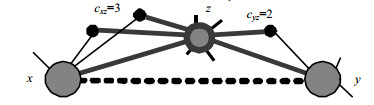
Here, the $\delta (\delta \geqslant 0)$ aims to adjust the strength of effectiveness. When $\delta {\rm{ = }}0$, the ECN index is the same as the CN index 12. TakeFig.1for example, the similarity of two endpoints is $s_{xy}^{{\rm{ECN}}} = ({3^\delta } + {2^\delta })/{9^\delta }$.

Figure 1. Effectiveness of common neighbors between two endpoints.
-
To quantify the prediction accuracy, the standard metric called precision[27]is introduced. Precision is defined as the ratio of relevant links to the top L predicted links (here we set L=100). If there are m relevant links appeared in the probe set, the precision value is:
Clearly, the higher precision value means higher prediction accuracy.
Our experiments are performed on fifteen different real networks: 1) Jazz[28]:the network of Jazz musicians. 2) Caenorhabditis elegans (CE)[29]: the neural network of the nematode worm. 3) Kohonen[30]: the citing network of articles with topic "self-organizing maps" or references to "Kohonen T". 4) USAir[31]: the USA airline network. 5) Hamster[32]: a friendship network of users on the website hamsterster.com. 6) Metabolic[33]: the metabolic network of Caenorhabditis elegans. 7) Email network (Email)[34]: the internal email communication network between employees of a mid-sized manufacturing company. 8) Yeast PPI (Yeast)[35]: a protein-protein interaction network of yeast. 9) Political blogs (PB)[36]: a network of US political blogs. 10) Openflights (Flight)[37]: the network of flights between air-ports of the world. 11) Scientometrics (SciMet)[30]: the citing network of the articles from scientometrics. 12) Food Web of Everglades ecosystem (FWEW)[38]: the network of carbon exchanges occurring during the wet season in the Everglades Graminoid Marshes of South Florida. 13) Route topology of internet (Router)[39]: the topology of internet in router-level. 14) Power Grid (Power)[29]: an electrical power grid network of western US; 15) Food Web of Florida Bay ecosystem (FWFB)[38]: the network of carbon exchanges occurring during the wet season in Florida Bay.
Table 1 shows the basic topological features of these networks. $\left| V \right|$is the number of nodes, $\left| E \right|$ denotes the number of links, $\left\langle k \right\rangle $ indicates the average degree. $\left\langle d \right\rangle $denotes the average distance. r is the assortativity coefficient[40]. C represents the clustering coefficient[29]. H is the degree heterogeneity.
Data $\left| V \right|$ $\left| E \right|$ $\langle k\rangle $ $\langle d\rangle $ r C H Jazz 198 2 742 27.7 2.24 0.02 0.633 1.4 CE 297 2 148 14.46 2.46 -0.163 0.308 1.8 Kohonen 3 704 12 683 3.4 5.64 -0.121 0.252 11.2 USAir 332 2 128 12.81 2.74 -0.208 0.749 3.36 Hamster 1 858 12 534 13.49 3.39 -0.085 0.090 3.36 Metabolic 453 2 025 8.94 2.67 -0.226 0.647 4.49 Email 167 5 784 69.26 1.87 -0.295 0.541 1.66 Yeast 2 375 11 693 9.85 5.10 0.469 0.378 3.48 PB 1 222 16 717 27.36 2.74 -0.221 0.361 2.97 Flight 2 939 30 501 20.75 4.18 0.051 0.255 5.22 SciMet 3 084 10 399 6.74 4.18 -0.033 0.151 2.78 FWEW 69 880 25.51 1.64 -0.298 0.552 1.27 Router 5 022 6 258 2.49 5.99 -0.138 0.033 5.5 Power 4 941 6 594 2.67 18.9 0.003 0.107 1.45 FWFB 128 2 075 32.42 1.78 -0.112 0.335 1.24 Table 1. Basic topological features of real networks
Each original data is randomly divided into training set containing 90% of links, and the probe set containing the remaining 10%.
-
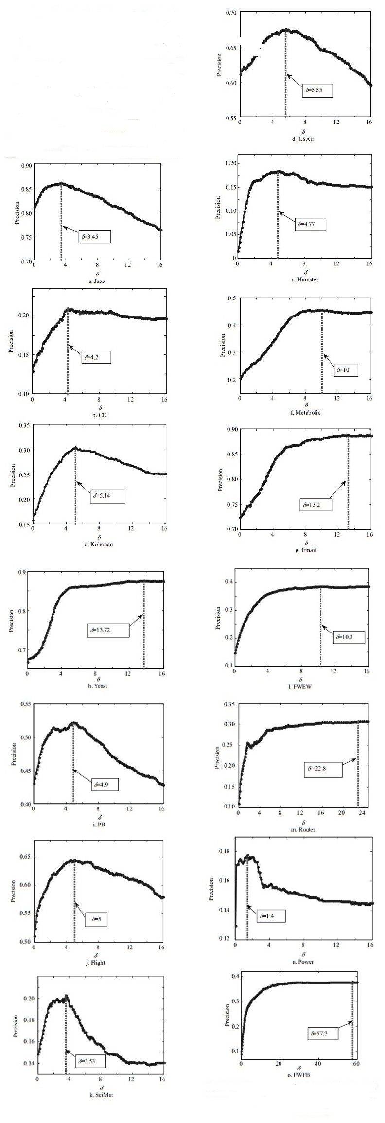
Firstly, we report the impact of adjust parameter$\delta $ on prediction accuracy in different networks, and each precision value is the average of 20 realizations. As shown in Fig. 2, all the precision curves can achieve the optimal values when $\delta > 1$, and each of them exceeds the precision value at $\delta = 1$ without enhancement. It demonstrates that higher effective neighbors have a much greater influence on the similarity between endpoints than expected and the contribution of different effective common neighbors for similarity is not linear (for different networks, its power exponent is the optimal $\delta $). The precision values show a rising trend with an increase of $\delta $ before reaching the highest point, which indicates that the effective common neighbors can improve the prediction accuracy compared with CN (when $\delta = 0$). The measurement of effective common neighbors and their enhancement are both beneficial to the description of similarity between two endpoints. For some of datasets, the precision curves decline gradually after peak point. However, the precision values are stable around the maximum value in some networks such as metabolic, Email, Yeast, FWEW, Router and FWFB. In these networks, the role that the lower effective common neighbors play is very limited in link prediction of missing links.
Table 2 shows the comparison between ECN index (optimal values) and 9 similarity indices in 15 networks, and each precision data is the average of 20 realizations. In 10 out of 15 datasets, ECN index obtains the best performance, but worse than the SPM index in Jazz, Hamster, PB, FWEW and FWFB. For some lower clustering network such as Hamster and Router, the improvement of precision is significant for ECN index, which indicates that common neighbors with different topological structures perform different roles in calculating the similarity between endpoints in these lower clustering networks. With the consideration of longer path information, the precision values of path-based indices (LP and Katz) are higher than neighbor-based indices (CN, RA and AA) in most of dataset. However, in some high clustering network such as Jazz, USAir, Metabolic and Email, the neighbor-weighted indices (RA and AA) perform better than most of the global indices. Also, the local- community-based index CAR can perform better than some global indices in Jazz, Kohonen, PB, Flight and SciMet. Having considered the effectiveness of common neighbors, ECN index can get a good performance by fusing some topology information used in neighbor-weighted indices and path-based indices. With the strength parameter, ECN index enhance the performance of effectiveness by adjusting the influence of different effective common neighbors on similarity in different networks. Having considered the structural consistency of a network, SPM performs very well for all the datasets. Surprisingly, some global indices (ACT and Cos+) perform worse than expected, and their precision values are close to zero in SciMet, Router, and Power networks. To summarize, the common neighbors between endpoints seem to be more effective for similarity calculating under the standard metric precision, and the consideration of local information around common neighbors can significantly improve the precision value.

Figure 2. Precision curves of ECN index with the change of parameter for 15 real networks. Each precision point is the average of 20 realizations
Data CN RA AA CAR LPa LPb Katza Katzb ACT Cos+ SPM ECN Jazz 0.810 0.809 0.830 0.851 0.798 0.775 0.798 0.740 0.258 0.356 0.895 0.861 CE 0.129 0.131 0.137 0.129 0.138 0.138 0.138 0.138 0.064 0.069 0.207 0.210 Kohonen 0.157 0.145 0.154 0.211 0.159 0.159 0.159 0.155 0.010 0.020 0.089 0.304 USAir 0.611 0.636 0.632 0.612 0.615 0.612 0.615 0.604 0.492 0.104 0.589 0.676 Hamster 0.015 0.004 0.011 0.037 0.017 0.054 0.017 0.075 0.089 0.020 0.898 0.186 Metabolic 0.206 0.305 0.253 0.195 0.201 0.200 0.201 0.200 0.120 0.110 0.445 0.456 Email 0.724 0.733 0.727 0.691 0.726 0.722 0.726 0.714 0.633 0.637 0.809 0.889 Yeast 0.668 0.495 0.693 0.670 0.671 0.733 0.670 0.721 0.565 0.239 0.699 0.876 PB 0.431 0.253 0.389 0.472 0.436 0.465 0.436 0.467 0.127 0.342 0.669 0.522 Flight 0.511 0.354 0.443 0.631 0.521 0.559 0.522 0.554 0.344 0.030 0.127 0.646 SciMet 0.149 0.130 0.147 0.165 0.149 0.150 0.149 0.147 0.000 0.000 0.079 0.203 FWEW 0.147 0.163 0.154 0.142 0.158 0.189 0.158 0.197 0.271 0.000 0.543 0.387 Router 0.110 0.092 0.113 0.109 0.132 0.132 0.131 0.130 0.000 0.019 0.015 0.306 Power 0.130 0.071 0.097 0.131 0.148 0.148 0.146 0.146 0.000 0.086 0.017 0.178 FWFB 0.090 0.087 0.086 0.089 0.096 0.133 0.096 0.146 0.178 0.030 0.718 0.378 aParameter $\alpha {\rm{ = 0}}{\rm{.001}}$. bParameter$\alpha {\rm{ = 0}}{\rm{.01}}$. Table 2. Comparison of the precision value between ECN (optimal value) and some similarity indices. Each value is the average of 20 realizations, each of which corresponds to an independent division of ${E^T}$and ${E^P}$
-
There are a lot of similarity indices considering local information between endpoints such as common neighbors and shorter paths. However, most of them ignore the effectiveness of common neighbors. Based on local information, an ECN index is proposed, which weights the common neighbors by the local topology information around them. Empirical results demonstrate that ECN index can significantly improve the prediction accuracy in 15 real networks, compared with 7 similarity indices. The measurement of effective common neighbors and their enhancement are both beneficial to the improvement of prediction accuracy or description of similarity between two endpoints. The ECN index is more suitable for the link prediction of networks concerning more about the prediction accuracy of the top L predicted links (such as protein-protein interaction networks). In addition, the complexity of ECN is between $O(N{\left\langle k \right\rangle ^2})$ (CN) and ${\rm{2}}O(N{\left\langle k \right\rangle ^2})$. Therefore, it can also be applied to predict missing links of large-scale networks.

 DownLoad: